Prediction Using

Regression Analysis

 Lots of Worked-Out, Easy-To-Understand, Graduate-Level Problems  --->
( Scroll Down and Take a Look ! )

 

Introduction

Multiple Regression Analysis is a statistical tool used to create predictive models. The Regression Equation - the end result of  Regression analysis - predicts the value of an output variable (the dependent variable) based upon the values of one or more input variables (the independent variables). The independent regression variables are sometimes called explanatory variables. The regression output consists of regression coefficients and regression variables as illustrated below. The regression model that results from regression testing is one of the most useful tools for the business manager.

Table of Contents

 Introduction
The Regression Equation
Simple Regression
Multiple Regression
Major Purposes of Linear Regression
Required Assumptions for Linear Regression
Creating the Regression Equation Using the Method of Least Squares
Creating the Regression Equation for a Two-Variable Regression
Creating the Regression Equation for a Three-Variable Regression
Creating the Regression Equation for a Multi-Variable Regression
The Steps for Performing Regression Analysis
   1) Graph the Data
   2) Perform Correlation Analysis Between All Variables
   3) Calculate the Regression Equation
   4) Calculate r square and Adjusted r square
   5) Calculate the Standard Error of Estimate
   6) Perform ANOVA
   7) Evaluate the Residuals
Estimated Standard Error of the Conditional Mean
Confidence Interval of Estimated Y Value
Multicollinearity
Homoscedasticity
Heteroscedasticity
Logistic Regression Analysis
Nonlinear Regression
The 7 Most Common Correctable Causes of Sample Data Appearing Non-Normal

Problem 1
Problem 2
Problem 3
Problem 4
Problem 5
Problem 6

The Regression Equation

The inputs for Regression Analysis are normally presented in a format similar to what is presented below:

When Regression Analysis is run on the above data, the output of the Regression, the Regression Equation, will have the following form:

 Y = B0 + (B1 * X1) + (B2 * X2) + (B3 * X3) + (B4 * X4)

B0, B1, B2, B3, and B4 are Coefficients of the Regression Equation.

This Regression Equation allows you to predict a new output (the dependent variable Y) based upon a new set of inputs (the independent variables X1, X2, X3, and X4).

The above was an example of a multiple regression using 5 variables.

 

Simple Regression

Very Basic Definition of Linear Regression Two-Variable – or Simple - Regression - The simplest type of regression has one dependent variable (usually Y) and one independent variable (usually X).
This is called two-variable regression. The regression equation for the two variable regression has the following form

Yest = B0 + (B1 * X1)

B0 and B1 are Coefficients of a two-variable Regression Equation.

Yest = B0 + (B1 * X1) is the formula of a straight line with a y-intercept of B0 and a slope of B1. The point (X1,Yest) lies somewhere directly on this regression line.

If we know X1, then we can calculate Yest, which is a value lying on the regression line and having an X value of X1.

The regression equation is calculated from a sample of points ( Xi ,Yi ). Each of these points lies somewhere around the regression line:
Yest = B0 + (B1 * X1).

The difference between the actual Y value of the sampled point and estimated Y value calculated by plugging in the sample’s X value into the regression
equation is called the residual or error.

The actual Y value is referred to as Y. The value of Y can be formulated as follows:

Y1 = B0 + (B1 * X1) + Error1

 

Multiple Regression

Multiple Regression - Regression with more than one independent variable is called Multiple Regression. The simplest type of multiple regression uses one dependent variable and two independent variables. This is a three-variable regression and has a regression equation with the following form:

Y = B0 + (B1 * X1) + (B2 * X2)

B0, B1, and B2 are Coefficients of a three-variable Regression Equation.

The Least Squares Method of Linear Regression

 

Major Purposes of Linear Regression Analysis

1. To provide a method of estimating the values of dependent variables from independent variables. The values of independent variables can be plugged into the Regression Equation to provide an estimate of the dependent variable.
2. To determine which independent variables have the greatest effect upon the output (the dependent variable). The magnitude of each regression coefficient indicates the degree of effect that variable has upon the output. The scale upon which each independent variable is measured must be accounted for when stating which variables have the greatest effect upon the output dependent variable.
3. To evaluate the error, or residual values, between the actual sampled values of the independent variable (Y) and the estimated values of the independent variable (Yest).
4. To evaluate how well the sampled points fit the linear regression equation line. In other words, to evaluate the goodness of fit between between the actual sampled values of the independent variable (Y) and their corresponding estimated values of the independent variable (Yest), all of which fall on the regression line.
5. To evaluate how statistically significant the overall regression equation is and also how statistically significantly significant each regression coefficient is. An output is statistically significant if it can be shown to not have occurred by chance.

 

Required Assumptions for Linear Regression Analysis

1. The sample taken must be representative of the population.
2. The general relationship between sampled points must be linear. For a two-variable regression, a scatter plot of all sampled values will visually show whether the sampled points generally fall near a straight line or not. For multi-variable regression, the goodness of fit (the degree of linearity or how well the sampled points fit the Regression Equation Line) is displayed by a statistic called the Standard Error of the Regression. This is part of the regression analysis output. Much more on this later.
3. The independent variables must be error-free.
4. The independent variables must independent of each other. It must not be possible to predict any independent variable from the value of one or more of the other independent variables.
5. The independent variables should not be highly correlated with each other. This will cause a condition known as multicollinearity.
6. If any of the input variables are categorical, then dummy variable techniques must be included in the regression analysis. A categorical independent variable would be, for example, set to 1 if a product color was red and set to 2 if a product color was blue.
7. The dependent variable must be continuous. Dependent variables that are discontinuous or categorical require advanced regression techniques such as logistic regression. These techniques are not discussed in this course. An example of a categorical dependent variable would be a regression in which the independent variables (the X’s) measured attributes of customers and the dependent variable (the Y’s) were set to a value of 1 if the customer bought and 0 if the customer did not buy. Logistic regression would be used to create a regression equation for this problem.
8. The average residual value should be 0.
9. The variance the residuals of should be constant throughout all input values. This is a condition called homoscedasticity. When the variance of the residuals is not constant, this is a condition called heteroscedasticity. Much more on this later.
10. All residuals should be independent.
11. All residuals should be normally distributed. This is an important assumption and can generally be met if at least 30 sample points are taken

Linear Regression Error of Extrapolation

 

Creating the Regression Equation Using

the Method of Least Squares

The method of Least Squares is used to calculate the regression equation. The method of Least Squares minimizes Σ(Y - Yest)²

 

Creating the Regression Equation for a

Two-Variable Regression

For a two-variable regression, the least squares regression line is:

Yest = B0 + (B1 * X)

The regression coefficient B0 B1 for a two-variable regression can be solved by the following “Normal Equations” :

B1 = (ΣXY – n*Xavg*Yavg) / (ΣX2 – n*Xavg*Xavg)

B0 = Yavg – B1*Xavg

Here is an example:

X	Y	XY	X2
1	4	4	1
2	7	14	4
3	8	24	9
4	13	52	16
10	32	94	30
ΣX	ΣY	ΣXY	ΣX2

Xavg = ΣX / n = 10 / 4 = 2.5

Yavg = ΣY / n = 32 / 4 = 8

B1 = (ΣXY – n*Xavg*Yavg) / (ΣX2 – n*Xavg*Xavg)

B1 = (94 – 4*2.5*8) / (30 – 4*2.5*2.5) = (94 – 80) / (30 – 25) = 2.8

B0 = Yavg – B1*Xavg

B0 = 8 – (2.8)*(2.5) = 1

Yest = B0 + (B1 * X)

Yest = 1 + (2.8 * X)

 

Creating the Regression Equation for a

Three-Variable Regression

For a three-variable regression, the least squares regression line is:

Yest = B0 + (B1 * X1) + (B2 * X2)

The regression coefficient B0 B1 B2 for a two-variable regression can be solved by the following Normal Equations using linear algebra techniques:

ΣY = nB0 + B1ΣX1 + B2ΣX2

ΣX1Y = B0ΣX1 + B1ΣX12 + B2ΣX1X2

ΣX2Y = B0ΣX2 + B1ΣX1X2 + B2ΣX22

 

Linear Regression Error of Extrapolation

 

Creating the Regression Equation for a

Multi-Variable Regression

If more than three variables exist in a regression equation, solving it by hand would be extremely cumbersome. This analysis can be easily performed in Microsoft Excel. In fact, any regression analysis, even two-variable regression, is solved much quicker with Excel than by hand.

 

The Steps to Performing Regression Analysis:

1. Graph The Data, If It Is A Two-Variable Regression.
2. Perform Correlation Analysis Between All Variables.
3. Calculate The Regression Equation.
4. Calculate r2 And Adjusted r2
5. Calculate The Standard Error Of Estimate
6. Perform ANOVA Analysis
7. Graph And Analyze The Residuals

Below is a completed example. We will use the data sample points of the previous example:

It is possible, but a bit cumbersome, to perform all regression calculations by hand for a two-variable regression. Linear regressions of all sizes can be quickly analyzed in Microsoft Excel. Below are all of the calculations of two-variable regression analysis based upon the above data.

 

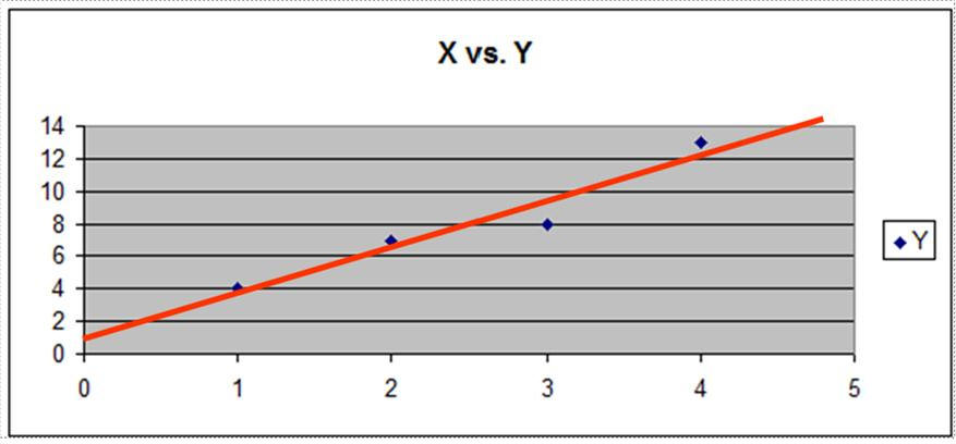
1) Graph the Data, if it is a two-variable regression. It is a two-variable regression and the scatter plot graph appears as follows:

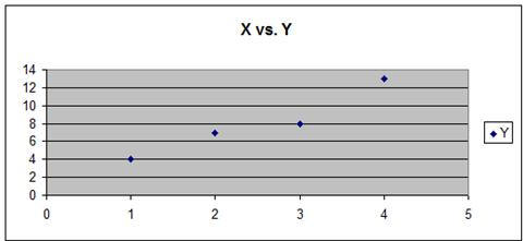
Visual inspection of the graph shows that there is a linear relationship between the data points. They appear to fall around line.

 

2) Perform Correlation Analysis Between All Variables.

The relationship between any two groups of sampled values is called the Sample Correlation Coefficient. It is sometimes also called the Pearson Correlation Coefficient. Its formula is as follows:

Sample Correlation Coefficient = rxy

rxy = [ n* ΣXY – ΣX*ΣY ] / [ SQRT(n*ΣX2 – (ΣX)2) * SQRT ( n*ΣY2 – (ΣY)2 ) ]

The main purpose of performing correlation analysis determine if any independent variables are highly correlated with each and determine as a result which independent variable to discard.

The two data series that are being correlated are as follows:

They need to be arranged in following way to facilitate correlation analysis:

	X	Y	XY	X2	Y2
	1	4	4	1	16
	2	7	14	4	49
	3	8	24	9	64
	4	13	52	16	169
Totals	10	32	94	30	298
	ΣX	ΣY	ΣXY	ΣX2	ΣY2

 

Number of samples = n = 4

Xavg = ΣX / n = 10 / 4 = 2.5

Yavg = ΣY / n = 32 / 4 = 8

rxy = Correlation Coefficient between X and Y

rxy = [ n* ΣXY – ΣX*ΣY ] / [ SQRT(n*ΣX2 – (ΣX)2) * SQRT ( n*Σy2 – (Σy)2 ) ]

rxy = [ 4*94 – 10*32 ] / [ SQRT(4*30 – (10)2) * SQRT ( 4* 298 – (32)2 ) ]

rxy = 0.966

If there are more than two variables in the regression, correlation analysis should be performed between each variable and every other variable, both independent and dependent. Performing a complete correlation analysis between multiple sets of variables can be easily and quickly implemented using Microsoft Excel.

It is very important that the independent variables are independent of each other. It should not be possible to predict one independent variable from one or
any combination of independent variables. No independent variables should be highly correlated with any other independent variables. An error called
multicollinearity occurs if any of the above conditions are true. If two independent variables are highly correlated, keep that independent variable which is
most highly correlated with the dependent variable and discard the other independent variable.

The main purpose of performing correlation analysis determine if any independent variables are highly correlated with each and determine as a result which independent variable to discard. In a two-variable regression, there is only a single independent variable. In a regression with three or more variables, there will be at least two independent variables. In this case, there is a possibility of independent variables that are highly correlated.

 

3) Calculate The Regression Equation.

The data should be arranged as follows to facilitate the analysis:

Xavg = ΣX / n = 10 / 4 = 2.5

Yavg = ΣY / n = 32 / 4 = 8

B1 = (ΣXY – n*Xavg*Yavg) / (ΣX2 – n*Xavg*Xavg)

B1 = (94 – 4*2.5*8) / (30 – 4*2.5*2.5) = (94 – 80) / (30 – 25) = 2.8

B0 = Yavg – B1*Xavg

B0 = 8 – (2.8)*(2.5) = 1

Yest = B0 + (B1 * X)

Yest = 1 + (2.8 * X)

For a linear regression having more than two variables, it is much easier to use software to create the regression equation and instead of doing the calculations by hand. Microsoft Excel has an excellent tool for creating linear regression equations with large numbers of independent variables.

 

4) Calculate r Square and Adjusted r Square

 r Square explains what percentage of total variance of the output (dependent variable) is explained by the variance of the inputs (independent variables). In other
words, r Square represents the proportion of the total variation that is explained by the regression equation.

 

Total Variance = Explained Variance + Unexplained Variance

Σ (Y – Yavg)2       = Σ (Yest – Yavg)2         + Σ (Y – Yest)2

r Square = Sample Coefficient of Determination

r Square = Explained Variance / Total Variance

Since Total Variance = Explained Variance + Unexplained Variance

Σ (Y – Yavg)2                 = Σ (Yest – Yavg)2           + Σ (Y – Yest)2

 

r Square = Explained Variance / Total Variance

r Square = 1 - [ Unexplained Variance / Total Variance ]

r Square = 1 - [ Σ (Y – Yest)2 / Σ(Y – Yavg)2 ]

	X	Y	Yest	(Y-Yest)2	(Y-Yavg)2
	1	4	3.8	0.04	15
	2	7	6.6	0.16	1
	3	8	9.4	1.98	0
	4	13	12.2	0.64	25
Totals	10	32	32	2.8	42

 

r Square = 1 - [ Σ (Y – Yest)2 / Σ(Y – Yavg)2 ]

r Square = 1 - [ 2.8 / 42 ] = 0.9333

This indicates that 93.33% of the total variance is explained by the regression equation. Only 6.667% of the total variance is unexplained.

Adjusted r Square

Adjusted r Square is an adjustment of r Square that takes into account the number of explanatory terms in a linear regression model. Adding a new independent variable to the regression model will improve Adjusted r Square only if the new term provides more explanatory power to the model. Adjusted r Square will always be equal to or less than r Square and Adjusted r Square can be negative. For a regression equation having 2 independent variables, Adjusted r Square is calculated by the following formula:

 

Adjusted r Square = 1 - [ {Σ (Y – Yest)2 / (n-2)} / {Σ(Y – Yavg)2 / (n-1)} ]

Adjusted r Square = 1 - [ {2.8 / (4-2)} / {42 / (4-1)} ] = 0.9

For a regression equation having any number of independent variables, Adjusted r Square is calculated by the following formula:

Adjusted r Square = 1 - [ {Σ (Y – Yest)2 / (n-k)} / {Σ(Y – Yavg)2 / (n-1)} ]

n = number of observations

k = Number of independent variables

 

5) Calculate The Standard Error Of Estimate

The standard error of estimate indicates the degree of scatter of the observed y values around the estimated y values on the regression line and is given by the equation:

sy.12…(k-1) = Standard error of the Estimate for a regression with any number of variables.

sy.12…(k-1) = SQRT [ Σ(Y – Yest)2 / (n-k) ]

n = number of observations

k = number of constants in the regression equation

sy.x = Standard error of the Estimate for a two-variable regression is:

sy.x = SQRT [ Σ(Y – Yest)2 / (n-k) ]

In this case, n = 4 and k = 2, therefore:

sy.x = SQRT [ 2.8 / (4-2) ] = SQRT [ 1.4 ] = 1.1832

6) Perform ANOVA Analysis

Analysis of Variance, ANOVA, evaluates the significance of the overall regression equation. ANOVA answers the question of whether the output of the regression analysis - the regression equation – is statistically significant or not. The basic question that ANOVA answers is the following: How likely is it that the coefficients of the regression equation are representative of what the true coefficients should be and not just randomly-generated numbers? ANOVA answers this question by performing a hypothesis test on a Null Hypothesis which states that the regression equation has no predictive power.

ANOVA performs this Hypothesis test using an F distribution. This Hypothesis test will be described in further detail below but can be summarized briefly as follows:

An F statistic is calculated for this regression model based upon the how the total variation proportioned between Explained and Unexplained Variation and also the degrees of freedom that this regression model has. The model’s F statistic is then compared with the critical F statistic. If the model’s F statistic is smaller than the critical F statistic, then we cannot reject the Null Hypothesis which states that the regression equation has no predictive power. If the model’s F statistic is larger than the critical F statistic, then we reject the Null Hypothesis and accept the Alternate Hypothesis which sates that the regression equation does have predictive power.

To sum up the above:

Test the overall significance of the regression equation by applying the following two rules;

1) If F(ѵ1, ѵ2) > Fα , the regression is significant

2) If F(ѵ1, ѵ2) ≤ Fα , the regression is not significant

F(ѵ1, ѵ2) = the Model’s F statistic and will be explained shortly

Fα = Critical F Statistic for the given α and will be explained shortly

Details of how this Hypothesis test is performed using the F distribution are shown as follows:

ANOVA is derived from the following relationship that is the basis of the calculation of r2:

Total Variance = Explained Variance + Unexplained Variance

Σ (Y – Yavg)2       = Σ (Yest – Yavg)2         + Σ (Y – Yest)2

 

The Explained Variance is often referred to the Regression Sum of Squares.

The Unexplained Variance is referred to as the Error Sum of Squares or the Residual Sum of Squares.

Source of	Sum of	Degrees of	Mean
Variation	Squares	Freedom	Squares
Regression	Σ(Yest – Yavg)2	ѵ1 = k -1	Σ(Yest – Yavg)2/(k - 1)
Error	Σ(Y – Yest)2	ѵ2 = n - k	Σ(Y – Yest)2/(n - k)
Total	Σ(Y – Yavg)2	n – 1

k = the number of constants in the regression equation. For example, if the regression equation is of the form

Yest = B0 + (B1 * X1) + (B2 * X2) --> There are 3 constants in this regression equation.

So k = 3.

n = the number of observations. If the sample includes five data points, then n = 5.

From the above information, the model’s F statistic is calculated as follows:

F(ѵ1, ѵ2) =	Σ(Yest – Yavg)2 * (k -1)
	Σ(Y – Yest)2 * (n - k)

A regression model’s F statistic is always calculated this way regardless of the number of variables that are in the equation.

The model’s F statistic is then compared with the critical F value, Fα (F “alpha”). This critical F value, Fα , can be located on an F distribution chart and is based upon the specified level of certainty required and also upon the same degrees of freedom, ѵ1 and ѵ2, as the model’s F statistic. If the model’s F statistic is larger than the critical F value, the regression model is said to be statistically significant.

Following are the calculations of the model’s F statistic and the critical F value for the current problem:

The Explained Variation is often referred to the Regression Sum of Squares.

The Unexplained Variation is referred to as the Error Sum of Squares or the Residual Sum of Squares.

Source of	Sum of	Degrees of	Mean
Variation	Squares	Freedom	Squares
Regression	Σ(Yest – Yavg)2	ѵ1 = k -1	Σ(Yest – Yavg)2/(k - 1)
Error	Σ(Y – Yest)2	ѵ2 = n - k	Σ(Y – Yest)2/(n - k)
Total	Σ(Y – Yavg)2	n – 1

k = the number of constants in the regression equation. For example, if the regression equation is of the form

Yest = B0 + (B1 * X1) + (B2 * X2) --> There are 3 constants in this regression equation.

So k = 3.

n = the number of observations. If the sample includes five data points, then n = 5.

From the above information, the model’s F statistic is calculated as follows:

F(ѵ1, ѵ2) =	Σ(Yest – Yavg)2 * (k -1)
	Σ(Y – Yest)2 * (n - k)

Here are the actual calculations from the current problem:

	X	Y	Yest	(Y-Yest)2	(Yest-Yavg)2
	1	4	3.8	0.04	17.64
	2	7	6.6	0.16	1.96
	3	8	9.4	1.98	1.96
	4	13	12.2	0.64	17.64
Totals	10	32	32	2.8	39.2
	ΣX	ΣY	ΣYest2	Σ(Y – Yest)2	Σ(Yest – Yavg)2

Yavg = ΣY / n = 32 / 4 = 8

k = number of constants in the regression equation = 2

n = number of observations = 4

ѵ1 = k -1 = 1

ѵ2 = n – k = 2

******************************************************************

Source of	Sum of	Degrees of	Mean
Variation	Squares	Freedom	Squares
Regression	Σ(Yest – Yavg)2	ѵ1 = k -1	Σ(Yest – Yavg)2/(k - 1)
Error	Σ(Y – Yest)2	ѵ2 = n - k	Σ(Y – Yest)2/(n - k)
Total	Σ(Y – Yavg)2	n – 1

******************************************************************

Source of	Sum of	Degrees of	Mean
Variation	Squares	Freedom	Squares
Regression	39.2	ѵ1 = 1	39.2
Error	2.8	ѵ2 = 2	1,4
Total	42	3

******************************************************************

F(ѵ1, ѵ2) =	Σ(Yest – Yavg)2 * (k -1)	=  39.2	= 28
	Σ(Y – Yest)2 * (n - k)	1.4

The Model’s F Statistic = F(ѵ1=1, ѵ2=2) = 28

******************************************************************

The Critical F Statistic for (ѵ1=1, ѵ2=2) equals Fα(ѵ1=1, ѵ2=2) and depends upon the required Level of Significance, α. If a 95% Level of Certainty is required, then the Level of Significance, α, = 5%, or 0.05.

This Critical F Statistic is found on the F distribution chart in the location corresponding to the correct ѵ1, ѵ2, and Level of Significance.

If α = 0.05, ѵ1=1, and ѵ2=2, then Fα=0.05(ѵ1=1, ѵ2=2) = 18.51

******************************************************************

The Model’s F Statistic = F(ѵ1=1, ѵ2=2) = 28

The Critical F Statistic = Fα=0.05(ѵ1=1, ѵ2=2) = 18.51

 

Decision Rule:

If the model’s F statistic is smaller than the critical F statistic, then we cannot reject the Null Hypothesis which states that the regression equation has no predictive power.

If the model’s F statistic is larger than the critical F statistic, then we reject the Null Hypothesis and accept the Alternate Hypothesis which sates that the regression equation does have predictive power.

In this case, the Model’s F Statistic is greater than the Critical F Statistic for α = 0.05. We therefore state there is at least 95% probability that the regression model is statistically significant.

******************************************************************

The Model’s F Statistic’s p value is the area under the F distribution curve that is outside of the Model’s F statistic.

The area under the F distribution curve that is outside of the Critical F Statistic will be equal to α. If α = 0.05, then 5% of the total area under the F distribution curve will be outside of the Critical F Statistic.

If the Model’s F Statistic is greater than the Critical F Statistic, the Model’s F Statistic’s p value will be less than α.

 

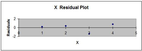
7) Evaluate the Residuals – Visually inspect a graph of the residuals to ensure that none of the following rules concerning residual are violated:

1. The average residual value should be 0.
2. The variance the residuals of should be constant throughout all input values. This is a condition called homoscedasticity. When the variance of the residuals is not constant, this is a condition called heteroscedasticity. More on this later.
3. All residuals should be independent.
4. All residuals should be normally distributed. This is an important assumption and can generally be met if at least 30 sample points are taken.

Following is a plot of the residuals from the current problem. The residual requirements appear to be met.

 

Estimated Standard Error of the Conditional Mean

The Estimated Standard Error of the Conditional Mean ( syest ) is used when calculating a Confidence Interval for the estimated Y value from a regression equation. For example, a 95% Confidence Interval for a specific regression output, Yest , is in interval in which we are 95% sure that the true regression output actually resides. The formula for this Confidence Interval is as follows:

95% Confidence Interval = Yest +/- Z 95%,2-tailed * syest

syest = sy.x * SQRT [ 1/n + (X0 – Xavg)2 / (ΣX2 – (ΣX)2/n) ]

One note on using the normal distribution instead of the t distribution for this type of problem: The t distribution is often used when performing statistic analysis on small samples (n < 30). An absolute requirement for this is that the underlying population from which the sample was drawn must be Normally distributed. This can never be assumed.

One way to circumvent this issue is to simply take a sample size larger than 30. Large sample sizes can be statistically analyzed using the Normal or t distributions even if the underlying population is not Normally distributed.

Statistics’ most fundamental theorem, the Central Limits Theorem, states this. When sample size is larger than 30, the t distribution become nearly identical to the Normal distribution. The Normal distribution is simpler to use because it does not require the degrees of freedom parameter that the t distribution requires.

In a nutshell, take sample sizes larger than 30 and use the Normal distribution for statistical analysis. It’s just easier, and isn’t that the point -----> to make things as simple as possible, but correct.

Multicollinearity

Multicollinearity is a regression error that occurs when there is a high correlation between independent variables.  This often occurs when too many independent variables are introduced into the regression equation at once. Regression equations should be built up slowly. Correlation analysis should be run between any potential new independent variable and all existing independent variables. A new variable that is highly correlated with an existing independent variable should not be added.

Multicollinearity manifests itself when new independent variables are added by causing large or unintuitive changes in the coefficients of existing independent variables in the regression equation while increasing explained variance (Adjusted r2) by only a small amount.

Always perform correlation analysis before adding new independent variables. Add new independent variables one at a time and observe the over-all effect before adding an additional independent variable.

Homoscedasticity

One important assumption of regression analysis is that there is the same amount of spread or variance about the regression line for each value of the independent variables. In most cases, the residuals can be visually observed to determine whether or not the required homoscedasticity exists.

Residuals are the individual differences between calculated value of the dependent variable (usually Y) and their actual values. These residuals are mapped along an X-Y axis. Homoscedasticity exists if the residuals are randomly spread about the X-axis with no bias or pattern. In this case, there is minimal explanatory power in the residuals.

Heteroscedasticity

Heteroscedasticity occurs when patterns or bias can be observed in the mapping of the residuals. When this happens, some of the model's explanatory power comes from the residuals.

 

Problem 1

A sales director of a large company wants to determine the relationship between the amount of time her salespeople spend prospecting and the amount of sales that they generate. She randomly sampled monthly sales results and monthly hours of prospecting for 30 salespeople from a sales force of over 1,000 salespeople. Below are the results of this random sample:

A) Derive the linear regression equation relating monthly sales (Y) to the monthly hours of prospecting (X). Predict the monthly sales for each employee’s hours of prospecting listed above.

B) Estimate the monthly sales for a salesperson who has prospected that month for 82 hours.

The random sample is as follows:

Xavg = ΣX / n = 85.75

Yavg = ΣY / n = 7

B1 = (ΣXY – n*Xavg*Yavg) / (ΣX2 – n*Xavg*Xavg)

B1 = 0.099

B0 = Yavg – B1*Xavg

B0 = -1.485

Yest = B0 + (B1 * X)

Yest = -1.485+ 0.099 * X

 

Predict the monthly sales for each employee’s hours of prospecting listed above.

 

B) Estimate the monthly sales for a salesperson who has prospected that month for 82 hours.

Yest = -1.485 + 0.099 * X

Yest = -1.485 + 0.099 * (82)

Yest = 6.629

 

Problem 2

A production line station can be operated at different speeds produces a varying number of defects every hour. With the station operating at different speeds, a simple random sample of 50 hour-long observations was selected.

X = speed of the production station in meters per second (mps)

Y = number of defects produced by the station during each observed hour.

n = 50

ΣX = 677

ΣY = 256

ΣXY = 15799

ΣX2 = 15888

a) Derive the linear regression equation

b) The station was operating at 15 mps during one hour. Estimate the number of defects during that hour.

Derive the linear regression equation

Xavg = ΣX / n  =  677 / 50  =  13.54

Yavg = ΣY / n  =  256 / 50  =   5.12

B1 = (ΣXY – n*Xavg*Yavg) / (ΣX2 – n*Xavg*Xavg)

B1 = 1.8348

B0 = Yavg – B1*Xavg

B0 = -19.7237

Yest = B0 + (B1 * X)

Yest = -19.7237 + 1.8348 * X

Calculate the expected number of defects per hour if the station is operated at 15 mps.

Yest = -19.7237 + 1.8348 * X

Yest = -19.7237 + 1.8348 * (15)

Yest = 7.7989

 

Problem 3

An economist wants to determine how accurately a company's annual marketing expenses can be predicted based upon the company's gross sales over the past year. The economist surveyed a representative, random sample of 15 firms and obtained their gross sales and marketing expenses figures for the previous year. For this problem, at least 30 samples should have been taken, but, for brevity, only 15 were taken. Perform the following calculations based upon the sample data below:

a) Estimate the linear regression equation using gross sales as the independent variable and marketing expense as the dependent variable.

b) Calculate the standard error estimate, sy.x.

c) Obtain the 95% confidence interval for marketing expenses for $130M of gross income.

d) Calculate Total Variance, Explained Variance, and Unexplained Variance

Below is the sample data:

a) Estimate the linear regression equation using gross sales as the independent variable and marketing expense as the dependent variable.

 

Xavg = ΣX / n  =  3059/15  =   203.93

Yavg = ΣY / n  =  1426 / 15  =   95.06

B1 = (ΣXY– n*Xavg*Xavg) / (ΣX2 – n*Xavg*Xavg)

B1 = 0.43

B0 = Yavg – B1*Xavg

B0 = 7.28

Yest = B0 + (B1 * X)

Yest = 7.28 + 0.43*X

 

 

b) Calculate the standard error estimate, sy.x.

 

b) Calculate the standard error estimate, sy.x.

sy.x = SQRT [ Σ(Y – Yest)2 / (n-2) ]

sy.x = SQRT [ 8609.57 / (15-2) ]  =  25.73

sy.x = 25.73

 

c) Obtain the 95% confidence interval of marketing expenses for $130M of gross sales

95% confidence interval of marketing expenses for $130M gross sales =

= Yest +/- Z95%,2-tailed * syest

X = 130

Yest = 63.24

Z95%,2-tailed = 1.96

syest = sy.x * SQRT [ 1/n + (X0 – Xavg) / (ΣX2 (ΣX)2/n) ]

syest = 0.557

95% confidence interval for $130M income = Yest +/- Z95%,2-tailed * syest

95% confidence interval for $130M income = 63.24 +/- 0.557

= 62.68 to 63.80 ($millions)

 

d) Calculate Total Variance, Explained Variance, and Unexplained Variance

Total Variance   =   Explained Variance   +   Unexplained Variance

Σ (Y – Yavg)2      = Σ (Yest – Yavg)2           +   Σ (Y – Yest)2

Total Variance = Σ (Y – Yavg)2 = 34536.93

Explained Variance = Σ (Yest – Yavg)2 = 25927.37

Unexplained Variance = Σ (Y – Yest)2 = 8609.57

 

Problem 4

Regression analysis was performed on data that was derived from 58 samples. The following 3 pieces of information were provided:

n = 58

Σ(Y - Yest)2 = 3600

Σ(Y - Yavg)2 = 19500

From the above data, solve the following tasks:

a) Calculate the Error of Estimate, sy.x

sy.x = SQRT [ Σ(Y – Yest)2 / (n-2) ]

sy.x = 8.02 ($millions)

sy.x = measures the scatter of the actual y values around the computed ones.

 

b) Calculate the Unadjusted coefficient of determination

r Square = 1 - ( Σ(Y - Yest)2 / Σ(Y - Yavg)2 )

r Square = 0.815

 

Now calculate the Adjusted coefficient of determination

Adjusted r Square = 1 - [ ( Σ(Y - Yest)2 / Σ(Y - Yavg)2 ) * ( (n-1) / (n-2) ) ]

Adjusted r Square = 0.812

r Square is the percentage of variability explained by the regression equation.

 

d) Calculate Total variance, Explained Variance, and Unexplained Variance;

Total Variance = Explained Variance + Unexplained Variance

Σ (Y – Yavg)2      = Σ (Yest – Yavg)2           +   Σ (Y – Yest)2

19500 = Σ (Yest – Yavg)2 + 3600

Σ (Yest – Yavg)2 = 15900

Total Variance = Σ (Y – Yavg)2 = 19500

Explained Variance = Σ (Yest – Yavg)2 = 15900

Unexplained Variance = Σ (Y – Yest)2 = 3600

 

 

Problem 5

Regression analysis was performed with the following variables:

Independent Variable = Y

Dependent Variables = X1 and X2

Y = Annual Gross Sales of Sampled Company

X1 = Size of Product Line (Number of Products) Sold by Sampled Company

X2 = Number of Salespeople Employed in Sampled Company

n = Number of Companies Sampled

 

103 random companies (n = 103) were sampled and provided the information for variables Y, X1, and X2. A regression was run on the sampled information and the following regression output was obtained:

		Regression
Variable	Mean	Coefficient
X1	11.75	0.079
X2	3.865	0.058

Intercept = 0.69

 

Analysis of Variance Table

	Sum of	Degrees of
Source	Squares	Freedom
Regression	1179.542	2
Error	397.678	100
Total	1577.22

 

a) Calculate and interpret the coefficient of multiple determination adjusted for degrees of freedom (Adjusted r2).

b) Estimate the Gross Sales of a company that has 12 products and 6 salespeople.

c) Test the overall significance of the regression using a 1% level of significance.

d) Calculate the Standard Error of Estimate

 

a) Calculate and interpret the coefficient of multiple determination adjusted for degrees of freedom (Adjusted r Square).

Adjusted r Square = 1 - [ {Σ (Y – Yest)2 / (n-k)} / {Σ(Y – Yavg)2 / (n-1)} ]

 

	Sum of
Source	Squares
Regression	1179.542	= Σ(Yest - Yavg)2
Error	397.678	= Σ(Y - Yest)2
Total	1577.22	= Σ(Y - Yavg)2

		Regression
Variable	Mean	Coefficient
X1	11.75	0.079
X2	3.865	0.058

Intercept = 0.69

B0 = 0.69

B1 = 0.079

B2 = 0.058

3 Independent Variable = B0, B1, B2

k = Number of Constants = 3

n = Number of Samples = 103

Regression Equation is as follows:

Yest = B0 + (B1 * X1) + (B2 * X2)

Yest = 0.69 + 0.079 * X1 + 0.058 * X2

	Sum of	Degrees of
Source	Squares	Freedom
Regression	1179.542	2	= k - 1
Error	397.678	100	= n - k
Total	1577.22

 

Σ(Y-Yest)2 = 397.678

Σ(Y-Yavg)2 = 1577.22

n - k = 100

n-1 = 102

Adjusted r Square = 1 - [ {Σ (Y – Yest)2 / (n-k)} / {Σ(Y – Yavg)2 / (n-1)} ]

Adjusted r Square = 1 - [ {397.678 / 100} / {1577.22 / 102} ]

Adjusted r Square = 0.743

74.3% of the Variance of Y is explained by the regression equation.

 

b) Estimate the Gross Sales of a company that has 12 products and 6 salespeople.

X1 = 12

X2 = 6

Yest = 0.69   +   0.079 * X1   +   0.058 * X2 = 1.986 ($M) Gross Sales

 

c) Test the overall significance of the regression using a 1% level of significance.

Test the overall significance of the regression equation by applying the following two rules;

1)      If F(ѵ1, ѵ2) > Fα , the regression is significant

2)      If F(ѵ1, ѵ2) ≤ Fα , the regression is not significant

ѵ1 = k - 1 = 2

ѵ2 = n - k = 100

α = 0.01

F(ѵ1, ѵ2) =	Σ(Yest – Yavg)2 * (k -1)
	Σ(Y – Yest)2 * (n - k)

F(ѵ1, ѵ2) = 148.30

Critical F Value = Fα = Fα=0.05(ѵ1=2, ѵ2=100) = 4.82

F(ѵ1, ѵ2) > Fα , therefore the regression is significant

 

d) Calculate the Standard Error of Estimate

sy.12…(k-1) = Standard Error of the Estimate for a regression having any number of variables

sy.12…(k-1) = SQRT [ Σ(Y – Yest)2 / (n-k) ]

n = number of observations

k = number of constants in the regression equation.

sy.12 = Standard Error of the Estimate for a regression having 2 independent variables

sy.12 = 1.994

This quantity can be thought of as the standard deviation of the dispersion of sample values about the estimated Y value.  

 

Problem 6

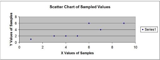
For this following set of points:

a)  Graph the above points

b)  Find the Least Square Regression Line

c)   Calculate the Standard Error of Estimate.

d)   Determine how many points are within 1 standard error from the regression line.

e)   Find the Coefficient of Determination Adjusted for Degrees of Freedom (Adjusted r Square)

f)   Find the Correlation Coefficient between X and Y

 

 

a)  Graph the above points

 

b)  Find the Least Square Regression Line

Arrange the data as follows:

Xavg = ΣX / n = 5

Yavg = ΣY / n = 3.286

B1 = (ΣXY – n*Xavg*Yavg) / (ΣX2 – n*Xavg*Xavg)

B1 = 0.667

B0 = Yavg – B1*Xavg

B0 = -0.048

Yest = B0 + (B1 * X)

Yest = -0.048+ 0.667* X

 

c)      Calculate the Standard Error of Estimate.

sy.12…(k-1) = Standard Error of the Estimate for a regression having any number of variables

sy.12…(k-1) = SQRT [ Σ(Y – Yest)2 / (n-k) ]

n = number of observations = 7

k = number of constants in the regression equation = 2

sy.x = Standard Error of the Estimate for a regression having 1 independent variable

sy.x = 1.163

 

d) Determine how many points are within 1 standard error from the regression line.

Number of points within 1 standard deviation of Yest = 5

 

d) Find the Coefficient of Determination (r2)

Yavg = 3.286

Σ (Y – Yest)2 = 6.76

Σ(Y – Yavg)2 ] = 45.72

r2 = 1 - [ Σ (Y – Yest)2 / Σ(Y – Yavg)2 ]

r2 = 0.8521

 

e) Find the Coefficient of Determination Adjusted for Degrees of Freedom (Adjusted r Square)

Adjusted r Square = 1 - [ {Σ (Y – Yest)2 / (n-k)} / {Σ(Y – Yavg)2 / (n-1)} ]

n = Number of observations = 7

k = Number of independent variables = 2

Adjusted r Square = 0.8225

 

f) Find the Correlation Coefficient between X and Y

Correlation Coefficient = r = SQRT(r Square) = 0.9231

The Correlation Coefficient measures the direction and magnitude of linear relationship between 2 variables.

r Square, the Coefficient of Determination, is more easily understood because it is a percentage.

r, the Correlation Coefficient, is not a percentage.

 

If You Like This, Then Share It...

 

 

 

Copyright   2013