|
|


| Normal (X, µ, σ2) = | ||||||
| λ | µ | σ | X | Poisson (X, λ) | Normal (X, λ, λ) | |
| 0.4 | 400 | 240 | 385 | 0.0153 | 0.0151 | |
| 400 | 0.0199 | 0.0199 | ||||
| 415 | 0.0148 | 0.0151 |

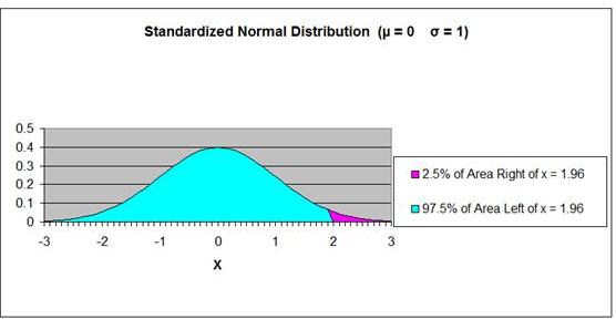
Problem 1: Using the Normal Distribution to Determine that Probability of Daily Production Level Will Be Below a Certain Point
A production machine has normally distributed daily output in units. The average daily output is 4000 and daily output standard deviation is 500. What is the probability that the production of one random day will be below 3580?
Problem Parameter Outline
Population Mean = µ = "mu" = 4,000
Population Standard Deviation =
σ = "sigma" = 500
x = 3,580
Probability x ≤ 3,580 = ?
Sales are Normally distributed
Normal curve is not standardized (µ ≠ 0,
σ ≠ 1)
Problem Solving Steps
We know that Production data is Normally distributed and
can therefore be mapped on the Normal curve.
We are trying to determine the probability that
Production Output will be below 3,580 units on any given
day.
This probability corresponds to the percentage of area
under the Normal curve that has an x value below (to the
left of) 3,580.
If we know how many standard deviations x = 3,580 is
from the mean (µ = 4,000),
we can use the Z Score Chart what percentage of total
area under the Normal curve is between x = 3,580 and the
mean.
Number of standard deviations x = 3,580 is from the mean
= Zx=3,580
z = (
x -
µ
) / σ
Zx=3,580 =
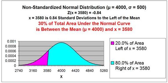
(3,580 - 4,000) / 500 = -0.84
The point x = 3,580 is 0.84 standard deviations from the
mean µ = 4,000. Because Zx=3,580
= -0.84 has a negative sign, that point is to the left
of the mean.
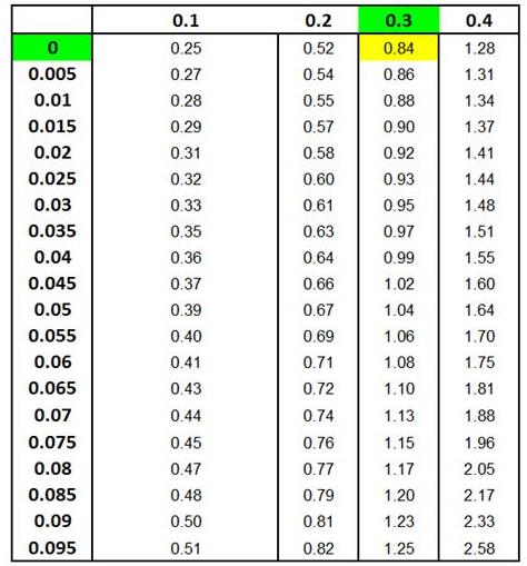
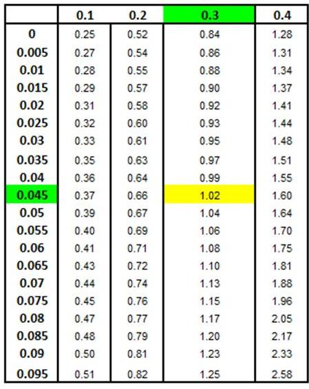
The Z
Score Chart below shows that 30% (0.30) of the total
area under the Normal curve will be between the mean and
a point that 0.84 standard deviations from the mean.
If 30% of the total area under the Normal curve is
between x = 3,580 and the mean
µ
= 4,000, then 20% of the total area under the
Normal curve must be outside this x value in the outer
left tail of the Normal curve, as is shown in the
graph of
the Normal curve below.
We obtain this percentage by subtracting 0.30 (30%) from
0.5. The mean divides the Normal curve in half and
each half on either side of the mean contains 50% of the
total area under the Normal curve.
This 20%
of the area under the Normal curve that is to the
left of x = 3,580 corresponds to the answer that that
there is 20% probability that the Production Level will
be less than 3,580 on any given day
Answer: There is a 20%
probability that the Production Level will fall below
3,580 units on any given day.
Z Score Chart
Z Score at x (Inner Numbers - Yellow)
vs.
Area Under Normal Curve
Between Mean (µ) and
x (Outer Numbers - Green)
Answer: There is a 20%
probability that the Production Level will fall
below 3,580 units on any given day.
This same problem above is solved in the Excel Statistical Master with only ONE Excel formula (and not having to looking anything up on a Z Chart). If you found your statistics book confusing, You'll really like the Excel Statistical Master. Everything is explained in simple, step-by-step frameworks.
Problem 2: Using the Normal Distribution to Determine the Probability that Daily Sales Will Be Within a Certain Range
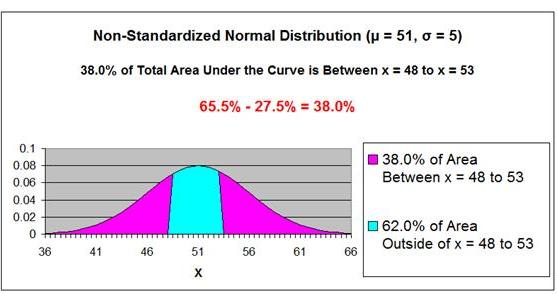
A salesperson has a mean daily sales of 51 units with a standard deviation of 5 units. What percentage of daily sales can be expected to be between 48 units AND 53 units? Weight is normally distributed for daily sales.
Problem Parameter Outline
Population Mean = µ = "mu" = 51 units
Population Standard Deviation =
σ = "sigma" = 5 units
48 units ≤ x ≤ 53 units
Probability that 43 ≤ x ≤ 53 = ?
units are Normally distributed
Normal curve is not standardized (µ ≠ 0,
σ ≠ 1)
Problem Solving Steps
We know that Daily Sales data is Normally distributed
and can therefore be mapped on the Normal curve.
We are trying to determine the probability that Daily
Sales will be between 48 and 53 on any given day.
This probability corresponds to the percentage of area
under the Normal curve that has an x value of 48 on the
lower (left) side and an x value of 53 on the upper
(right) side.
If we know how many standard deviations x = 48 and x =
53 each are from the mean (µ
= 50), we can use the Z Score Charts to find what
percentage of total area under the Normal curve is
between x = 48 and x = 53.
*****************************************************************
Number of standard deviations x = 48 is from the mean
= Zx=48
z = ( x - µ ) / σ
Zx=48 =
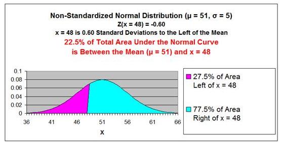
(48 - 50) / 5 = -0.60
The point x = 48 is 0.60 standard deviations from the
mean µ = 50. Because Zx=48
= -0.60 has a negative sign, that point is to the left
of the mean.
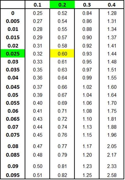
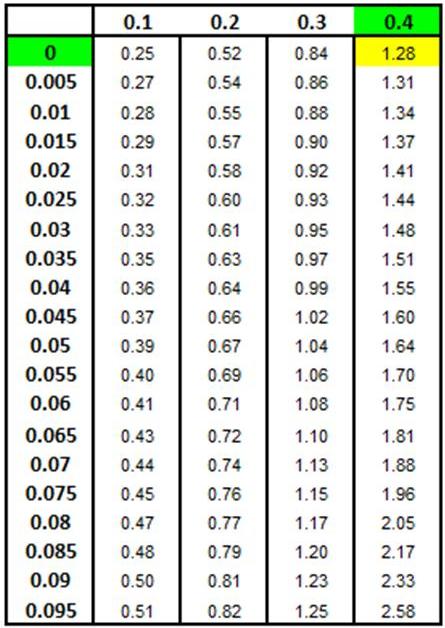
The 2nd
Z Score Chart below shows that 22.5% (0.225) of the
total area under the Normal curve will be between the
mean and a point (x = 48) that 0.60 standard deviations
from the mean.
If 22.5% of the total area under the Normal curve is
between x = 48 and the mean (x = 50), 27.5% of the total
area under the Normal curve must exist in the outer left
tail to the left of x = 48.
This is
illustrated in the 2nd graph below.
*****************************************************************
Number of standard deviations x = 53 is from the mean
= Zx=53
z = (
x -
µ
) / σ
Zx=53 =
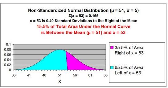
(53 - 50) / 5 = 0.40
The point x = 53 is 0.40 standard deviations from the
mean µ = 50. Because Zx=53
= 0.40 has a positive sign, that point is to the right
of the mean.
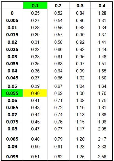
The 1st
Z Score Chart below shows that 15.5% (0.115) of the
total area under the Normal curve will be between the
mean and a point that 0.40 standard deviations from the
mean.
This is also shown in the 1st graph below.
if 15.5% of the total area under the Normal curve exists
between the point x = 53 and the mean, then 65.5% of the
total area under the Normal curve is to the left of the
point x = 53.
This is
also illustrated in the 1st graph shown below.
*****************************************************************
The total area under the Normal curve between x = 48 and
x = 53 equals the area to the left of
X = 53 (65.5%) MINUS the area to the left x = 48
(27.5%).
65.5% - 27.5% = 38%
38% of the total area under the Normal curve exists
between x = 48 and x = 53.
This is
shown in the 3rd graph below.
Answer: There is a 38%
probability that Daily Sales will fall between 48 units
and 53 units on any given day.
Z Score Chart
Z Score at x (Inner Numbers - Yellow)
vs.
Area Under Normal Curve
Between Mean (µ) and
x (Outer Numbers - Green)
EQUALS
Answer: There is a 38% probability that Daily Sales will fall between 48 units and 53 units on any given day.
This same problem is solved in the Excel Statistical Master with only 1 Quick Excel formula (and not haveing to look up ANYTHING on a Z Chart). The Excel Statistical Master teaches you everything in step-by-step frameworks. You'll never have to memorize any complicated statisical theory.
Problem 3: Using the Normal Distribution to Determine the Lower 10% Limit of Delivery Times
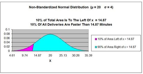
A pizza deliveryman's delivery time is normally distributed with a mean of 20 minutes and a standard deviation of 4 minutes. What delivery time will be beaten by only 10% of all deliveries?
Problem Parameter Outline
Population Mean = µ = "mu" = 20 minute
Population Standard Deviation =
σ = "sigma" = 4 minutes
x = ?
Probability that (delivery time ≤
x) = 10% = 0.10
Delivery time is Normally distributed
Normal curve is not standardized (µ ≠ 0,
σ ≠ 1)
Problem Solving Steps
We know that Delivery Time data is Normally distributed
and can therefore be mapped on the Normal curve.
We are trying to determine Delivery Time will be lower
than 90% of all Delivery Times.
This probability corresponds to the x value at which 90%
of area under the Normal curve has a greater value and
is to the right this x value. This x value must
therefore be in the left tail of the Normal curve.
If we know that 90% of the area under the Normal curve
is to the right of this x value (this is illustrated in
the graph
below), then we know that 40% of the total area
under the Normal curve is between this x value and the
mean. The remaining 50% of the area under the Normal
curve makes up the half the Normal curve that is on the
opposite side (the right side) of the mean.
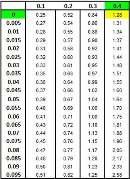
If we know that 40% of the area under the Normal curve
is between this x value and the mean, we can use the Z
Score Chart to determine how many standard deviations
this x value is from the mean. The
Z
Score Chart below shows this x value to be 1.28
standard deviations from the mean.
If we know how many standard deviations this x value is
from the mean, we can use the following formula to
calculate the x value, as follows:
z = (
x -
µ
) /
σ
x =
z *
σ +
µ
x = (-1.28) * 4 + 20 = 14.87
The delivery time of 14.87 minutes
is faster (smaller) than 90% of all delivery times.
This is
illustrated in the graph below.
Answer:
The delivery time of 14.87 minutes
is faster (smaller) than 90% of all delivery times.
Z Score Chart
Z Score at x (Inner Numbers - Yellow)
vs.
Area Under Normal Curve
Between Mean (µ) and
x (Outer
Numbers - Green)
Answer: The delivery time of 14.87 minutes is faster (smaller) than 90% of all delivery times.
This same problem is solved in the Excel Statistical Master with only 1 Excel formula (and not having to look up anything on a Z Chart - that's something you'll never have to do again with Excel). With the Excel Statistical Master you can do advanced business statistics without having to buy and learn expensive, complicated statistical software packages such as SyStat, MiniTab, SPSS, or SAS.
Problem 4: Using the Normal Distribution to Determine the Lower 10% Limit of Sales Bonuses
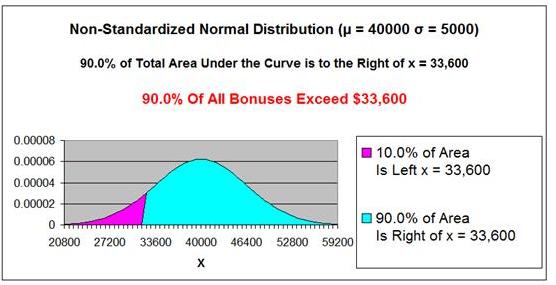
Salespeople of a large sales force received an annual bonus based upon performance. The size of the bonuses was Normally distributed with a mean of $40,000 and a standard deviation of $5000. What size bonus is exceeded by 90% of all other bonuses?
Problem Parameter Outline
Population Mean = µ = "mu" = $40,000
Population Standard Deviation =
σ = "sigma" =
$5,000
x = ?
Probability that (Bonus ≥
x) = 90% = 0.90
Bonus is Normally distributed
Normal curve is not standardized (µ ≠ 0,
σ ≠ 1)
Problem Solving Steps
We know that Bonus data is Normally distributed and can
therefore be mapped on the Normal curve.
We are trying to determine Bonus amount will be lower
than 90% of all other Bonuses.
This probability corresponds to the x value at which 90%
of area under the Normal curve has a greater value and
is to the right this x value. This x value must
therefore be in the left tail of the Normal curve.
If we know that 90% of the area under the Normal curve
is to the right of this x value (this is illustrated in
the graph
below), then we know that 40% of the total area
under the Normal curve is between this x value and the
mean. The remaining 50% of the area under the Normal
curve makes up the half the Normal curve that is on the
opposite side (the right side) of the mean.
If we know that 40% of the area under the Normal curve
is between this x value and the mean, we can use the Z
Score Chart to determine how many standard deviations
this x value is from the mean. The
Z Score
Chart below shows this x value to be 1.28 standard
deviations from the mean.
If we know how many standard deviations this x value is
from the mean, we can use the following formula to
calculate the x value, as follows:
z = (
x -
µ
) /
σ
x =
z *
σ +
µ
x = (-1.28) * 5,000 + 40,000 = 33,600
A Bonus of $33,600 smaller than
90% of all Bonus amounts.
This is
illustrated in the graph below.
Answer:
A Bonus of $33,600 smaller than
90% of all Bonus amounts.
Z Score Chart
Z Score at x (Inner Numbers - Yellow)
vs.
Area Under Normal Curve
Between Mean (µ) and
x (Outer
Numbers - Green)
Answer: A Bonus of $33,600 is smaller than 90% of all Bonus amounts.
This same problem is solved in the Excel Statistical Master with only 1 Excel formula (without having to look up anything on a Z Chart). If you found your statistics book confusing, You'll really like the Excel Statistical Master. Everything is explained in simple, step-by-step frameworks.
Problem 5: Using the Normal Distribution to Determine the Boundaries of the 75% Mid-Range of Sales Bonuses
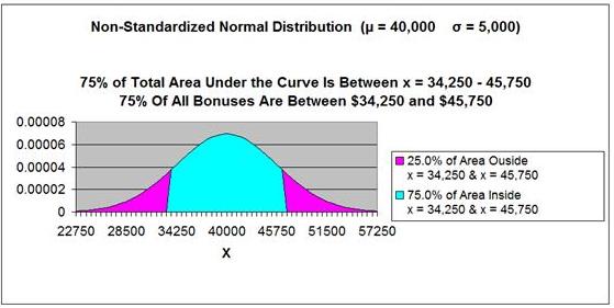
Salespeople of a large sales force received an annual bonus based upon performance. The size of the bonuses was Normally distributed with a mean of $40,000 and a standard deviation of $5000. What would be the mid range that 75% of all bonuses would be in?
Problem Parameter Outline
Population Mean = µ = "mu" = $40,000 miles
Population Standard Deviation =
σ = "sigma" = $5,000
x1 = ? x2 = ?
Left Boundary
Probability that (Bonus ≤ x1 ) = 12.5% = 0.125
And
Right Boundary
Probability that (Bonus ≤ x2 ) = 87.5% = 0.875
Bonus is Normally distributed
Normal curve is not standardized (µ ≠ 0,
σ ≠ 1)
Problem Solving Steps
We know that Bonus data is Normally distributed and can
therefore be mapped on the Normal curve.
We are trying to determine the range of Bonuses that
will be in the mid 75% of all Bonus amounts.12.5% of all
Bonuses will lower than this mid-range and 12.5 of all
Bonuses will be higher than this mid-range.
75% of all Bonuses corresponds to 75% of the area under
this Normal curve.
x1 is the x value in which 12.5% of all Bonuses (and
12.5% of the area under the Normal curve) is less than.
x1 exists in the outer left tail of the Normal curve.
This can be observed in the graph below.
x2 is the x value in which 12.5% of all Bonuses (and
12.5% of the area under the Normal curve) is greater
than than. x2 exists in the outer left tail of the
Normal curve. This can be observed in the graph below.
Both x1 and x2 each have 12.5% of the total Normal curve
area existing outside of their values. This means that
37.5% of the total area under the Normal curve exists
the mean and each x value. This can be observed from the
graph below.
The number of standard deviations between each x value
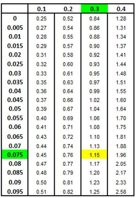
and the mean can be found on a Z Chart. The Z value for
the point that has 37.5% of the total curve area between
it and the mean is 1.15.
This
can be observed in the Z Chart below. zx1
= -1.15 and zx2
= 1.15. Each of these x values is therefore 1.15
standard deviations from the mean but on opposite sides
of the mean. This means that the two Z values will have
opposite signs.
If we know how many standard deviations (the Z Scores)
that these x value are from the mean, we can use the
following formula to calculate the x values, as follows:
z = (
x -
µ
) / σ
x =
z *
σ +
µ
x1 = (-1.15) * 5,000 + 40,000 = 34,250
x2 = 1.15 * 5,000 + 40,000 = 45,750
75% of all Bonuses fall between $34,250 and $45,750.
This can be observed on the graph below.
Answer: 75% of all
Bonuses fall between $34,250 and $45,750. This can be
observed on the graph below.
Z Score Chart
Z Score at x (Inner Numbers - Yellow)
vs.
Area Under Normal Curve
Between Mean (µ) and
x (Outer
Numbers - Green)
Answer: 75% of all Bonuses fall between $34,250 and $45,750. This can be observed on the graph below.
This same problem is solved in the Excel Statistical Master with only 2 Excel formulas (and never again having to look up anything on a Z Chart). The Excel Statistical Master will make you a fully functional statistician at your workplace.
Problem 6: Using the Normal Distribution to Determine the Probability that a Taxi Driver's Daily Mileage Will Be Within 1 of 2 Ranges
A large taxicab company analyzed the daily miles driven by each driver. The average distance was 200 miles with a standard deviation of 30 miles. A driver's mileage is selected at random. What is the probability that the this daily mileage will be either more than 261.5 mile OR less than 169.4 miles?
Problem Parameter Outline
Population Mean = µ = "mu" = 200 miles
Population Standard Deviation =
σ = "sigma" = 30 miles
169.4 miles ≥ x
OR
x ≥ 261.5 miles
Probability that 169.4 miles ≥ x
OR x ≥ 261.5 miles = ?
mileage is Normally distributed
Normal curve is not standardized (µ ≠ 0,
σ ≠ 1)
Problem Solving Steps
We know that Daily Mileage data is Normally distributed
and can therefore be mapped on the Normal curve.
We are trying to determine the probability that Daily
Mileage will be either be greater than 261.4
OR less than 169.4 miles on any
given day.
This probability corresponds to the percentage of area
under the Normal curve outside of (greater than or to
the right of) x1 = 261.5
PLUS the percentage of area under the
Normal curve outside of (less than or to the left of) x2
= 169.4.
This can be observed on the graph below.
We can calculate the Z values associated with each x
with this formula as follows:
z = (
x -
µ
) / σ
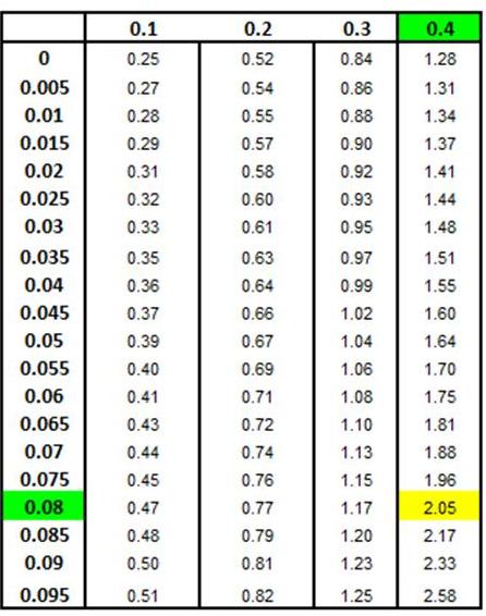
zx1 = (
261.5 - 200 ) / 30 = 2.05
zx2
= ( 169.4 - 200 ) / 30 = -1.02
Because we know the Z values associated with each x
value (zx1
and zx2),
we can determine how much curve area exists between each
x value and the mean.
The 1st
Z chart below shows that 48% of the total area under
the Normal curve exists between x1 and the mean.
This can
also be observed in the graph below.
The 2nd
Z chart below shows that 34.5% of the total area
under the Normal curve exists between x2 and the mean.
This can
also be observed in the graph below.
The total area under the Normal curve outside x = 261.5
and x = 169.4 equals the area outside of (to the right)
of
x = 261.5 (2% ---> 50% - 48% = 2%)
PLUS
the area outside of (to the left of) x = 169.4
(15.5% ---> 50% - 34.5% = 15.5%).
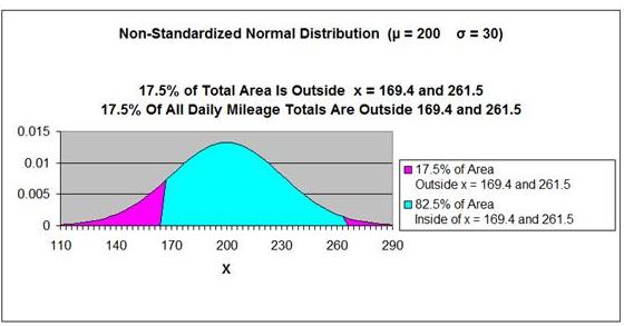
2% + 15.5% = 17.5%
17.5% of the total area under the Normal curve exists
outside of x = 261.5 and x = 169.4.
This is shown in the
graph below.
Answer: There is a 17.5%
probability that a taxi driver's Daily Mileage will be
greater than 261.5 or less than 169.4 miles on any given
day.
Z Score Chart
Z Score at x (Inner Numbers - Yellow)
vs.
Area Under Normal Curve
Between Mean (µ) and
x (Outer
Numbers - Green)
Answer: There is a 17.5% probability that a taxi driver's Daily Mileage will be greater than 261.5 or less than 169.4 miles on any given day.
This same problem is solved in the Excel Statistical Master with only 2 Excel formulas. The Excel Statistical Master is the fastest way for you to climb the business statistics learning curve.
Interesting Bit of Trivia
The Normal
Distribution is sometimes called the Gaussian
Distribution because a German mathematician named Karl
Gauss used the distribution to describe astronomical
data.
The last series of German 10 Mark notes displayed Karl
Gauss and the formula and graph of the Normal
Probability Density Function. Sehr Einer Guter Mann!
(What a good guy!)
Statistics in Excel Home Normal Distribution
t Distribution Binomial Distribution
Regression Confidence Intervals Combinations and Permutations
Correlation and Covariance ANOVA Other Useful Distributions
Statistical Training Videos
Statistics Blog
Statistics Jobs
Latest Manuals in the Excel Master Series
Contact Information Statistics Jobs
Internet Marketing Book Review
Blog EntriesUsing Logistic Regression in Excel To Predict If a Prospect Will Buy
Taguchi Testing - What Is It and Is It a Good For Landing Page Optimization?
How To Use the Chi-Square Independence Test in Excel to Figure Out What Makes Your Customers Buy More
How To Solve ALL Hypothesis Tests in Only 4 Steps
Statistical Mistakes You Don't Want To Make
A Quick Normality Test Easily Done in Excel
The 7 Most Common Correctable Causes of Sample Data Appearing Non-Normal
How To Use the t Test in Excel To Find Out If Your New Marketing Is Working
Using the Excel t Test To Find Out What Your Best Sales Days Are
Nonparametric Tests - Completed Examples in Excel
Nonparametric Tests - How To Do the 4 Most Important in Excel
Nonparametric Tests - When the Marketer Should Use Them
Using All 3 Types of ANOVA in Excel to Improve Your PPC Marketing
Comparing Doing ANOVA in Excel with Doing It By Hand
How To Use the Chi-Square Variance Test to Find Out If Your Customers Are Becoming More or Less Focused In Their Spending
Using ANOVA in Excel to Increase Click-Through Rate
The Two Crucial Steps to Excel Regression That Most People Skip
How To Quickly Read the Output of Excel Regression
Work-Arounds for Excel 2003 and Excel 2007s Biggest Statistical Omissions
How To Build a Better Split-Tester in Excel Than the Google Website Optimizer
How To Use Dummy Variable Regression in Excel to Perform Conjoint Analysis
The Chi-Square Goodness-of-Fit Test - Excel's Easiest Normality Test
The Mann-Whitney U Test Done in Excel
The Kruskal-Wallis Test Done in Excel
The Spearman Correlation Coefficient Test Done in Excel
The Sign Test (Nonparametric) Done in Excel
The Wilcoxon Rank Sum Test Done in Excel
The Wilcoxon Signed-Rank Test for Small Samples Done in Excel
The Wilcoxon Signed-Rank Test for Large Samples Done in Excel
Excel's Most Basic Forecasting Tool - The Simple Moving Average
The Weighted Moving Average - A Basic and Accurate Excel Forecasting Tool
Excel Forecasting Tool #3 - Exponential Smoothing
Normal Distribution's 4 Most Important Excel Functions
Using the Normal Distribution To Find Your Sales Limits
Using the Hypothesis Test in Excel To Find Out If Your Advertising Worked
Using the Hypothesis Test in Excel To Find Out If Your Delivery Time Worsened
Using the Hypothesis Test in Excel To Test Your Headlines
Creating a Confidence Interval in Excel To find Your Customer Preferences
Creating a Confidence Interval in Excel To Find Your Real Daily Sales
Using the Normal Distribution To Find Your Range of Daily Sales
SPC Control Charts in Excel - Done Properly
Excel Model Building - Experts vs. Non-experts
Using the Excel Solver To Optimize Your Internet Marketing Budget
Is SPC Limited By The Central Limit Theorem?
Top 10 SEO Excel Functions - You'll Like These!
How To Use the Excel Solver to Find Your Sales Curve
How To Use If-Then-Else In Excel To Remove Matches From 2 Lists
How To Use VLOOKUP In Excel To Find Matches From 2 Lists In 2 Steps
Pivot Tables - How To Set Up Pivot Tables Correctly Every Time
Pivot Tables - One Easy Step That Will Double the Effectiveness of All of Your Pivot Tables!
VLOOKUP - Just Like Looking Up a Number In The Telephone Book
VLOOKUP - Looking Up a Quantity Discount in a Distant Excel Spreadsheet With VLOOKUP
Statistical Training Videos
How To Use Logistic Regression in Excel To Predict If Your Prospect Will Buy
How To Use the Chi-Square Independence Test in Excel to Find Out What Makes Your Customer Make Bigger Orders
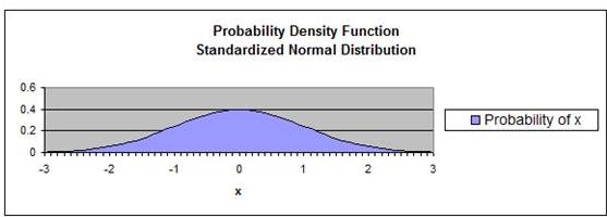
How to Graph the Normal Distribution's Probability Density Function in Excel
How To Use Dummy Variable Regression in Excel to Perform Conjoint Analysis
How To Use All 3 Built-In Types of ANOVA in Excel to Improve PPC Marketing
How To Use the Chi-Square Variance Test in Excel to Find Out If Your Customers Are More Focused In Their Spending
How To Create a Histogram and Pareto Chart in Excel
How To Improve a Twitter Follower Acquisition Program with a Histogram in Excel
How To Use SocialOomph - The Most Versatile and Popular Tweet Automation Tool
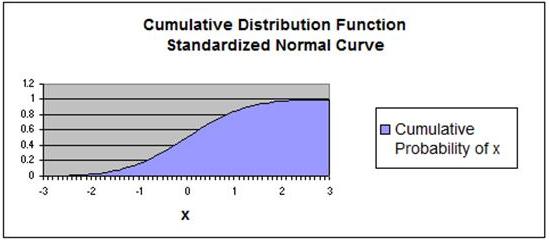
How To Graph the Normal Distribution's Cumulative Distribution Function in Excel
How to Build a Better Split-Tester in Excel Than the Google Website Optimizer
How To Do the 4 Steps to Regression in Excel - Including the 2 Crucial Steps That Are Almost Always Ignored
Excel Regression Output - How to Quickly Read and Understand It
How To Use ANOVA in Excel to Increase Click-Through Rate in a Pay-Per-Click Campaign
How To Do ANOVA in Excel and also by Hand - Single-Factor ANOVA
Work-Arounds for Excel 2003 and Excel 2007's Biggest Statistical Omissions
How To Graph the Students t Distributions' Probability Density Function in Excel
How To Graph the Chi-Square Distribution's Probability Density Function in Excel
How To Graph the Weibull Distribution's PDF and CDF - in Excel
How To Add Followers To Your Twitter Account Faster Than You Thought Possible
How To Solve Problems with the Weibull Distribution in Excel
How To Solve Problems with the Gamma Distribution in Excel
Copyright 2013