Other Useful Distributions
Lots of Worked-Out,
Easy-To-Understand, Graduate-Level Problems --->
( Scroll Down and Take a Look ! )
In additional to the
Normal, t, and Binomial distributions, there are a number of other useful
distributions that are commonly used to solve statistical problems that occur in
business.
Multinomial Distribution
Multinomial Distribution Problem 1 -
Calculate the probability of a combination of specified outputs for a given
number of independent trials
Hypergeometric Distribution
Hypergeometric Problem 1 - Calculate exact number of occurrences of an event
that occurs without replacement - Uses Hypergeometric Distribution
Hypergeometric Problem
2 - Calculate exact number of occurrences of an event
that occurs with replacement - Uses Binomial Distribution
Poisson Distribution
Poison Distribution Problem 1 - Calculate the
probability of an exact number of Poisson-distributed event occurring
Poison Distribution Problem 2 - Calculate the
probability of up to a certain number of Poisson-distributed event occurring
Uniform Distribution
Uniform Distribution Problem 1 - Calculate the
probability that a 2 or a 5 will appear with one roll of a fair die
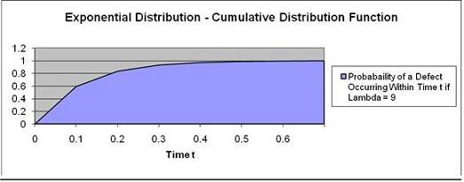
Exponential Distribution
Exponential Distribution Problem 1 -
Calculate the probability of an exponentially-distributed event (a defect in
a production line) occurring within a certain time.
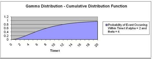
Gamma Distribution
Gamma Distribution Problem 1 - Calculate the
probability of Poisson-distributed event occurring before a certain time
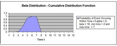
Beta Distribution
Beta Distribution Problem 1 - Calculate the
probability of an event occurring within a certain time for a given Alpha
and Beta along with min and max completion times
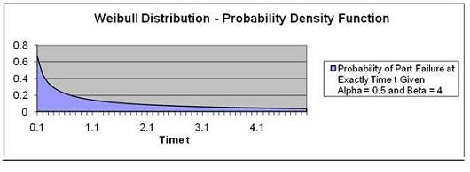
Weibull Distribution
Weibull Distribution Problem 1 - Calculate the
probability of a Weibull-distributed event (part failure) occurring at a
certain time
Weibull Distribution Problem 2 - Calculate the
probability of a Weibull-distributed event (part failure) occurring by a
certain time
F Distribution

The Multinomial Distribution is a generalization of the well-known Binomial
Distribution.
Like the Binomial Distribution, the Multinomial Distribution is a Discrete
distribution, not a Continuous distribution. This means that the objects
that form the distribution are whole, individual objects. This distribution
curve is not smooth but moves abruptly from one level to the next in
increments of whole units.
The Multinomial Distribution provides the probability of a combination of
specified outputs for a given number of trials that are totally independent.
The probability of each of the individual outputs of each of the trials must
be known in order to utilize the Multinomial Distribution to calculate the
probability of that unique combination of outputs occurring in the given
trials.
Here is the formula for calculating the probability of a multinomial
distribution:
P ( X1 = n1, X2 = n2, … ,
Xk = nk ) =
= [
(n!) /
(n1! * n2! * … *nk!)
]
* [Pr(X1 = n1)]n1
* [Pr(X2 = n2)]n2 *
...
... * [Pr(Xk = nk)]nk
The following example makes the Multinomial Distribution
easier to understand.
Problem: A box contains 5 red marbles, 4 white marbles,
and 3 blue marbles. A marble is selected at random, its
color noted, and then the marble is replaced. 6 marbles
are selected in this manner. Find the probability that
out of those 6 marbles, 3 are red, 2 are white,
and 1 is blue.
Total number of marbles = 12
n = total number of drawings = 6
X1 = Count of red marbles drawn = n1 = 3
X2 = Count of white marbles drawn = n2 = 2
X3 = Count of blue marbles drawn = n3 = 1
The probability of 3 red, 2 white, 1 blue = P(3 red, 2
white, 1 blue)
= P ( X1 = n1, X2 = n2, …, Xk = nk )
= P ( X1 = 3, X2 = 2, X3 = 3 )
P ( X1 = n1, X2 = n2, … ,
Xk = nk ) =
= [
(n!) /
(n1! * n2! * … *nk!)
]
* [Pr(X1 = n1)]n1
* [Pr(X2 = n2)]n2 *
...
... * [Pr(Xk = nk)]nk
= [ (6!)
/ (3! * 2! * 1! )
] * [5/12]3 *
[4/12]2 *
[3/12]1
= 625 / 5184 = 0.12056 = 12.06%
There is a 12.06% chance that, from a box containing 5
red marbles, 4 white marbles, and 3 blue marbles, from 6
marbles randomly selected, 3 are red, 2 are white,
and 1 is blue.
This same problem above is solved in the Excel Statistical Master with only 1 Excel formula. Everything is explained to you in SIMPLE language in the Excel Statistical Master.
When k = 2, the Multinomial Distribution is the Binomial
Distribution.
The
Hypergeometric Distribution is almost the same as
the Binomial Distribution, except that samples are
NOT
replaced back into the population. This is known as
Sampling Without Replacement.
The Binomial Distribution calculates the probability of
1 of 2 possible outcomes occurring a certain number of
times (x) in a certain number of independent trials (n).
The probability of the outcome occurring in a single
trial is known (p).
After each trial the samples ARE
replaced back into the population when using the
Binomial Distribution.
The Hypergeometric Distribution calculates the
probability of 1 of 2 possible outcomes occurring a
certain number of times (x) in a certain number of
independent trials (n). The probability of the outcome
occurring in a single trial is known (p).
After each trial the samples are NOT replaced back into
the population when using the Hypergeometric
Distribution.
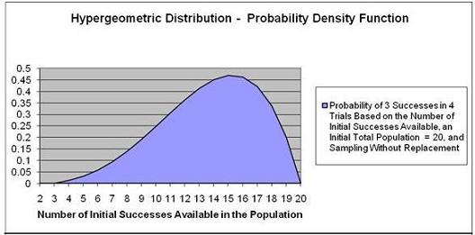
The problem below will illustrate the use of the
Hypergeometric Distribution formula:
Problem: A 20-piece chocolate sample consists of 8
caramel samples and 12 nut samples. Calculate the
probability that of 4 individual samples 3 taken will
produce caramels. Each sample is eaten (not replaced)
after it is taken. (If each
sample were replaced before the next sample was taken,
the Binomial distribution would be used)
Exact number of successes = 3
Number of trials = 4
Initial possible number of successes = 8
Initial population size = 20
There is a 13.87% probability that 3 out of 4 samples
taken without replacement will be caramel samples if the
box initially had 20 pieces of candy that included 8
caramel samples.
The y-value corresponding to the point
on the horizontal axis equaling 8 is 13.87%.
This same problem above is solved in the Excel Statistical Master with only 1 Excel formula. The Excel Statistical Master is the fastest way for you to climb the business statistics learning curve.
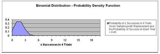
Problem:
If the above problem were the same except that you were
sampling with replacement (putting each candy back
instead of eating it before the next sample is taken),
it would solved with the Binomial Distribution as
follows:
This problem is solved using the Probability
Density Function and not the Cumulative Distribution
Function because we are solving for exactly 3 caramels
chosen in 4 trials, not up to 3 caramels.
There is 15.36% chance of
exactly 3 successes in 4 trials given Sampling with
Replacement and the Probability of Success on each trial
is 0.40.
Note that the graph at point 3 on the Horizontal has a y
value (probability) = 0.1536.
This same problem above is solved in the Excel Statistical Master with only 1 Excel formula. The Excel Statistical Master teaches you everything in step-by-step frameworks. You'll never have to memorize any complicated statisical theory.
The Poisson Distribution is a widely employed
distribution that is used to describe the probability of
events that are a result of a rate that occurs over time
such as:
Product demand
Demand for services
Number of telephone calls that come over a switchboard
Number of accidents
Number of traffic arrivals
Number of defects
The Poisson Distribution is a Discrete distribution.
This means that the events described by this function
occur in whole units. The graph of the Poisson
Distribution therefore moves from one level to the next
in discrete increments, not smoothly.
The Poisson Distribution is used to calculate the
probability of a certain number of specific events
occurring over a given period of time - if it is known
in advance that those events occur in frequency as
predicted by the Poisson Distribution. Previous
measurement must have been taken to determine: 1) that
the events occur in frequency according to the Poisson
Distribution, and 2) the average rate, which is the
expected number of occurrences of that event over the
given time period.
A problem will better illustrate the use of the Poisson
Distribution:
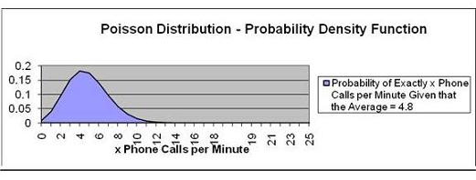
Problem: An average of 4.8 telephone calls per minute is
made through the central switchboard according to the
Poisson distribution. What is the probability that:
a) exactly 4 phone calls will be made in a given minute
Exact number of events = k = 4
Expected number of events = E(k)
Cumulative Distribution Function? No, Use the Probability Density
Function.
We want to calculate the probability of EXACTLY 4 phone
calls. This will be the
Probability Density Function, not the Cumulative
Distribution Function, which
would measure the probability of up to 4 phone calls
instead of exactly 4.
There is an 18.2% chance of
exactly 4 phone calls per minute.
Note that the point on the graph that has 4 as the value
on the horizontal axis has
a value of 0.182 on the vertical axis. The Poisson
distribution is a discrete distribution and not a
continuous distribution so the graph has corners at each
point instead of being smooth.
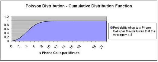
b) up to 4 phone calls will be made in a given minute
Exact number of events = k = 4
Expected number of events = E(k)
Cumulative Distribution Function? Yes
We want to calculate the probability of UP TO 4 phone
calls. This will be the
Cumulative Distribution Function.
Pr (Up To 4 Phone Calls) = Pr ( k = 4) = 47.6%
There is a 47.6% chance of up to
4 phone calls per minute.
Note that the point that represents up to 4 calls per
minute corresponds with 0.47 on the vertical axis.
This same Poisson problems as above are each solved in the Excel Statistical Master with only 1 Excel formula. With the Excel Statistical Master you'll never have to look up anything on a chart ever again.
A variable is uniformly distributed if all possible
outcomes of that variable have an equal probability of
occurring. For example, if a fair die has 6 possible
outcomes when rolled once, each outcome has the same 1/6
chance of occurring.
The Uniform Distribution is a Discrete distribution.
This means that its events described by this function
occur in whole units.
Problem: A fair die is rolled once. What is the
probability that either a 2 or a 5 will appear on top
after the roll?
Number of total possible outcomes in 1 trial = 6
Number of times that 2 appears as a possible outcome = 1
Number of times that 5 appears as a possible outcome = 1
Probability of a 2 occurring in 1 roll = 1/6 = 0.1667
Probability of a 2 occurring in 1 roll = 1/6 = 0.1667
Pr (2 occurs) OR Pr (5 occurs) = Pr (2 occurs) + Pr (5
occurs)
= 0.1667 + 0.1667 = 0.333 = 33.33% probability
There is a 33.33% probability
that either a 2 or a 5 will appear on top after the
roll.
The Exponential Distribution is used to calculate the
probability of occurrence of an event that is the result
of a continuous decaying or declining process. The
lengths between arrival times in a Poisson process could
be described with the
Exponential Distribution. Examples of arrival times
between Poisson events are as follows:
Time between telephone calls that come over a
switchboard
Time between accidents
Time between traffic arrivals
Time between defects
An example of a decaying process that would be predicted
by the Exponential Distribution would be:
Time until a radioactive particle decays
The Exponential Distribution is not appropriate for
predicting failure rates of devices or lifetimes of
organisms because a disproportionately high number of
failures occur in the very young and the very old. In
these cases, the distribution
curve would not be a smooth exponential curve as
described by the Exponential Distribution.
The Exponential Distribution predicts time between
Poisson events as follows:
Probability of length of time t between Poisson events =
f(t) = e-kt
k is sometimes called Lambda.
A problem will illustrate the use of this function:
Problem: A production machine has a very low defect
rate. Time between defects can be predicted by the
following Exponential Distribution function:
Time between failures (t) = f(t) = 9 e-9t
( t is measured in whole years )
Calculate the probability of a defect being produced
within the next 1/10th year.
(Using "Within" indicates that the Cumulative
Distribution function will be used)
t = 1/10 = 0.10
k = Lambda = 9
Use Cumulative Distribution Function? Yes
The probability of defect occurring in 1/10 years
is
59.34%
Note that the graph point at Time t = 0.1 has the
probability of 0.5934.
The Gamma Distribution represents the sum of n
exponentially distributed random variables. Applications
of the Gamma Distribution are often based on intervals
between Poisson-distributed events. Examples of these
would include queuing models, the flow of items through
manufacturing and distribution processes, and the load
on web servers and many forms of telecom.
Due to its moderately skewed profile, it can be used as
a model in a range of disciplines, including climatology
where it is a working model for rainfall, and financial
services where it has been used for modeling insurance
claims and the size of loan defaults. It has therefore
been used in probability of ruin and value-at-risk
equations.
The Gamma Distribution function is characterized by 2
variables, its shape parameter, alpha (α), and its scale
parameter, theta (Φ). The Gamma Distribution function
calculates the probability of wait time between Poisson
distributed events to be time t,
Problem: Calculate the probability of the a
Poisson-distributed event occurring before Time t = 10
if the Gamma Distribution function has alpha,
α, = 2 and
theta, Φ, = 4.
Units of waiting time until event occurs = t = 10
Alpha, α = 2
Theta, Φ = 4
Use the
Cumulative Distribution Function? Yes
The probability of this event occurring within 10 units of
time = 71.27%
Note that the graph point at Time t = 10 has a
probability of 0.7127.
This same problem above is solved in the Excel Statistical Master with only 1 Excel formula. The Excel Statistical Master will make you a fully functional statistician at your workplace.
The Chi-Squared Distribution is a Gamma distribution in
which the shape parameter,
α, is set to the degrees of
freedom divided by 2 and the scale parameter,
Φ, is set
to 2.
The Gamma Distribution with its shape parameter,
α, set
to 1 and its scale parameter,
Φ, set to b, becomes the
Exponential Distribution with k, lambda, set to b.
The Beta Distribution models events which are
constrained to take place between a minimum and maximum
time limit. For this reason, the Beta Distribution is
often used for modeling project planning and control
systems such as PERT (Project Evaluation and Review
Technique) and CPM (Critical Path Method). The Beta
Distribution is often used to calculate the probability
that a project will be completed within a given period of time. Below is an example which
illustrates its use:
Problem: Calculate the probability of completing the
following project before Time t = 5 if the project is
described by the following parameters:
Evaluation time period = t = 5
Alpha, α, = 8
Beta, ß, = 10
Minimum completion time in units of time = 2
Maximum completion time in units of time = 7
The probability of completing the task within time = 5 units
(within is a cumulative function) = 90.81%
Note that the graph point at Time t = 5 has a
probability of 0.908.
This same problem above is solved in the Excel Statistical Master with only 1 Excel formula. With the Excel Statistical Master you can do advanced business statistics without having to buy and learn expensive, complicated statistical software packages such as SyStat, MiniTab, SPSS, or SAS.
The Weibull Distribution is a special case of the
Generalized Extreme Value distribution. The Weibull
distribution has been used extensively as a model of
time to failure for manufactured items and has become
one of the principal tools of reliability engineering.
The applications of the Weibull Distribution have
expanded and include Finance and Climatology. There are
three parameters of the Weibull distribution: time t,
α
- alpha (the shape parameter), and
ß (the scale
parameter).
α > 1 --> Failure
rate increases over time (suggests "wear out")
α = 1 -->
Constant failure rate - Items fail from random events
α < 1 --> Failure
rate decreases over time (suggest high "infant
mortality")
Problem: Calculate the probability that a part will fail
at time = 2 if the part's failure occurrence is
Weibull-distributed and has a = 0.5 and ß = 4.
t = Time = 2
α = Alpha = 0.5
ß = Beta = 4
We are determining the probability of part failure at
exactly time t = 2 so we are using the Probability
Density Function.
The probability of part failure occurring at exactly Time t
= 2 ("exactly at" indicates using the Probability
Density Function) given that time to part failure is Weibull-distributed with a = 0.5 and ß = 4 is
calculated is 8.7%.
Note that the graph point at Time t = 2.0 has a
probability of 0.087.
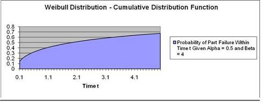
Problem: Calculate the
probability the a part will fail
by time = 2 if the part's
failure occurrence is
Weibull-distributed and has a =
0.5 and ß = 4.
Time t = 2
α = Alpha = 0.5
ß = Beta = 4
We are determining the
probability of part failure
by time t = 2 so
we are using the
Cumulative Distribution
Function.
The probability of part failure
occurring at exactly Time t = 2
given that time to part failure
is Weibull-distributed with
α = 0.5 and
ß = 4 is 50.6%.
This same Weibull Distribution problems as above are each solved in the Excel Statistical Master with only 1 Excel formula. You'll finally have a solid understanding of business statistics with the Excel Statistical Master.
The F Distribution is used to determine whether two
groups have different variances. The F Distribution is
normally used to develop confidence intervals and
hypothesis tests. It is rarely used for modeling
applications.
The F Distribution has 4 parameters:
Χ21
(the calculated Chi-Square statistic for data group 1),
Χ22
(the calculated Chi-Square statistic for data group 2),
ѵ1
(the degrees of freedom of group 1), and
ѵ2
(the degrees of freedom of group 2). An example of how
the Chi-Square statistic is calculated from a group of
data can be
found in the course module entitled "Chi-Square
Independence Test."
The F Distribution is actually a family of
distributions. Each different F Distribution has a
unique combination of ѵ1
and
ѵ2.
An individual F Distribution is actually the
distribution of the F Statistic. The formula for the F
Statistic is as follows:
F Statistic = ( Χ21
/
ѵ1)
/ (
Χ22
/
ѵ2)
As stated, the F Distribution is rarely used for
modeling applications, but is often used for developing
confidence intervals and hypothesis tests. Because of
this, the most important use of a particular F Statistic
is the calculation of its p Value. The p Value equals
the percentage of total area under that unique F
Distribution curve to the right of the given F statistic
(and therefore the area in the outer curve tail
to the right of the F Statistic).
The p Value is compared with a, the required Level of
Significance. If the p Value is less than
α, then the
two data groups are assumed to have different variances.
If the p Value is greater than
α, the two data
groups are assumed to have equal variances.
ANOVA testing is used to judge whether three or more groups have the same
mean (for example, same test scores) after each group has had a
different
treatment applied to it (for example, a different teaching method applied to
each group).
If there no real differences between the groups being tested, one would
expect that any measured differences between the groups would not be much
different than measured differences between samples taken from within
individual groups.
A F Ratio ( sometimes called an F Statistic) compares the differences
between groups to the differences within groups.
Conceptually, the F Ratio can be thought of as how different the means of
groups are relative to the variability within the groups. It might also be
helpful to view the following explanation:
| F Ratio = |
Real Differences +
Random Differences |
Between Groups |
| Random Differences |
Within Groups |
The actual definition of the F Ratio is as follows:
| F Ratio = |
Variance of the Group Means |
|
| Mean of the Within-Group Variances |
|
This is sometimes shortened to:
| F Ratio = |
Mean Square Between Groups |
|
| Mean Square Within-Group |
|
The larger the value of the F Ratio (sometimes called the F Statistic), the
greater the likelihood that the difference between groups is due to
Real Differences and not just
due to chance (
Random Differences).
The required degree of certainty (for example, we want to be at least 95%
that the groups are different) determines how large the F Ratio has to be
for us to be able to state that the groups are different.
The distribution of the F Ratio is called the F Distribution. The F
Distribution is a family of distributions, each described by the following
two parameters:
ѵ1 = Degrees of Freedom Between Groups
ѵ2 = Degrees of Freedom Within Groups
Critical F Values have been calculated for various degrees of certainty (99%
certainty, 95% certainty, etc.) for each of the basic F Distributions. The
general rule use to state whether real differences exists between groups for
a given level of certainty is as follows:
If F Statistic (ѵ1 , ѵ2) > F Critical
(ѵ1 , ѵ2)----> The different treatments affected the output
If F Statistic (ѵ1 , ѵ2) < F Critical
(ѵ1 , ѵ2)----> The different treatments did
not affect the output
The F Statistic and F Critical are calculated using the same ѵ1 and ѵ2. If
the F Statistic is greater than the F Critical that is calculated for a
specific degree of certainty, we can state that groups are statistically
different.
Calculating the F Statistic between two data sets
involves a lot of work. A complete example of the
calculation of the F Statistic between two
data sets is shown at the end of the ANOVA module. Here,
a hand-calculation of the F Statistic and p Value is
performed to determine if there is a relationship
between sales closing methods and sales results. The
problem required a 95% Level of Certainty. The
α (Level of
Significance) was therefore equal to 0.05. Sales results and
closing
methods are assumed to not be independent of each other
because different closing methods are shown to produce
different sales results.
A summary of that problem is as follows:
The problem requires determination of whether closing
methods used have an affect on sales. Three sales groups
were each required to use a different closing method for
the entire test. The total sales results from each group
were recorded. ANOVA analysis was employed to determine
with a 95% Level of Certainty whether the choice of
closing method affected the level of sales.
The ANOVA process breaks the data down in two ways for
analysis. One grouping of data is labeled the "Between
Groups" data. The other grouping of the
data is labeled the "Within Groups" data.
An F Statistic was
calculated based upon these two groups of data. The
calculated F Statistic was found to be greater than the
F Critical Value that was
based upon the 95% Level of Certainty. Therefore this
implies that sales are not independent of closing method
used. See the ANOVA module for the complete calculation.
A summary of the calculations is as follows:
"Between Groups" data grouping:
- Χ21
= Chi-Square StatisticGroup
1 = 72
- ѵ1
= degrees of freedomGroup
1 = 2
"Within Groups" data grouping:
- Χ22
= Chi-Square StatisticGroup
2 = 46
- ѵ2
= degrees of freedomGroup
2 = 9
F Statistic = ( Χ21
/
ѵ1)
/ (
Χ22
/
ѵ2)
= ( 72 / 2 ) / ( 46 / 9 )
= 7.04
| F Statistic(ѵ1
, ѵ2) ----> ѵ1 = DOF1
= 2, ѵ1 = DOF2
= 9 |
| F Statistic
(ѵ1=2,ѵ2=9) =
(MS Between Groups) / (MS Within Groups) |
|
F Statistic (ѵ1=2,ѵ2=9)
= 36 / 5.1 = |
7.04 |
F Criticalα=0.05(ѵ1=2,ѵ2=9)
= 4.265
If F Statistic (ѵ1 , ѵ2) > F Critical
(ѵ1 , ѵ2)----> The different treatments affected the output
If F Statistic (ѵ1 , ѵ2) < F Critical
(ѵ1 , ѵ2)----> The different treatments did
not affect the output
The calculated F Statistic(ѵ1 = 2,
ѵ2 = 9) = 7.04. This is greater than F Criticalα=0.05
(ѵ1 = 2, ѵ2 = 9) = 4.265.
This indicates that there is less than a 5% chance that
this result could have occurred if there was no
difference in the effectiveness between the closing
methods. Therefore, there is at least a 95% certainty
that there is a real difference in effectiveness of the
closing methods. The Null Hypothesis, which was
therefore rejected, states that choice of closing
methods does not affect sales.
The
p Value (which can be quickly calculated with Excel) = 0.0144
0.0144 is less than a (0.05) so
it is assumed that the two groups are not independent.
Sales are therefore related to the closing method used
because the variances are different.
Copyright 2013