The Confidence Interval
Lots of Worked-Out,
Easy-To-Understand, Graduate-Level Problems --->
( Scroll Down and Take a Look ! )
A Confidence Interval is an
estimate of a
population's average or
proportion based upon sample data drawn from the population.
A Confidence Interval is a range of values in which the mean
is likely to fall with a specified level of confidence or certainty.
Basic Explanation of Confidence Intervals
Mean Sampling vs. Proportion Sampling
Confidence Intervals of a Population Mean
Confidence Interval
Calculation Using Large Samples
The Central Limit Theorem
Levels of Confidence and Significance
Population Mean vs. Sample Mean
Standard Deviation and Standard Error
Region of Certainty vs. Region of Uncertainty
Z Score
Formula for Calculating Confidence Interval Boundaries from Sample Data
Confidence
Interval Desirable Properties of Data Sets
The 7 Most Common Correctable Causes of Sample Data Appearing Non-Normal
Problem 1: Calculate a Confidence Interval from a Random Sample of Test
Scores
Problem 2: Calculate a Confidence Interval of Daily Sales Based Upon Sample
Mean and Standard Deviation
Problem 3: Calculate an Exact Range of 95% of Sales Based Upon the
Population Mean and Standard Deviation
Determine Minimum Sample Size to Limit Confidence Interval of Mean to a
Certain Width
Problem 4: Determine the Minimum Number of Sales Territories to Sample
In Order To Limit the 95% Confidence Interval to a Certain Width
Confidence Interval
for a Population Proportion
Mean Sampling vs. Proportion Sampling
Levels of Confidence and Significance
Population Proportion vs. Sample Proportion
Standard Deviation and Standard Error
Region of Certainty vs. Region of Uncertainty
Z Score
Formula for Calculating Confidence Interval Boundaries from Sample Data
Problem 5: Determine Confidence Interval of Shoppers Who Prefer to Pay By
Credit Card Based Upon Sample Data
Determine Minimum Sample Size to Limit Confidence Interval of Proportion to a
Certain Width
Problem 6: Determine the Minimum Sample Size of Voters to be 95% Certain
that the Population Proportion is only 1% Different than Sample
Proportion


The Confidence Interval is an interval in which the true population
mean or proportion probably lies based upon a much smaller
random sample taken from that population.
Confidence Intervals for means are calculated differently than
Confidence Intervals for proportions. The first half of this course
module will discuss calculating a Confidence Interval for a
population mean. The second half will cover calculating a
Confidence Interval for a population proportion.
First we will briefly discuss the difference between sampling
for mean and sampling for proportion:
What determines whether a mean is being estimated or a
proportion is being estimated is the number of possible
outcomes of each sample taken.
Proportion samples have only two possible outcomes.
For example, if you are comparing the proportion of Republicans
in two different cities, each sample has only two possible values;
the person sampled either is a Republican or is not.
Mean samples have multiple possible outcomes.
For example, if you are comparing the mean age of people in two different
cities, each sample can have numerous
values; the person sampled could be anywhere from
1 to 110 years old.
Below is a description of how to calculate a Confidence
Interval for a population's mean. Note that everything is
almost the same as the calculation of the Confidence
Interval for a population proportion, except sample
standard error.
The Confidence Interval of a Mean is an interval in which
the true population mean probably lies based upon a
much smaller random sample taken from that population.
A 95% Confidence Interval of a Mean is the interval that
has a 95% chance of containing the true population mean.
The width of a Confidence Interval is affected by the
sample size. The larger the sample size, the more
accurate and tighter is the estimate of the true
population mean. The larger the sample size,
the smaller will be the Confidence Interval. Samples
taken must be random and also be representative of the
population.
Confidence Intervals are usually calculated and plotted
on a Normal curve. If the sample size is less then 30,
the population must be known to be Normally distributed.
If small-sample data (n<30) is used to plot the Confidence
Interval of the Mean for a population that is not Normally
distributed, the result can be totally wrong.
Probably the most common major mistake in statistics
is to apply Normal or t distribution tests to small-sample
data taken from a population of unknown distribution.
Typically the actual distribution of a population is not known.
If the population's underlying distribution is not known
(usually it is not), then only large samples (n>30) are
valid for creating a Confidence Interval of the Mean.
The most important theorem of statistics, the Central
Limit Theorem, explains the reason for this.
The Central Limit Theorem is statistics' most fundamental
theorem. In a nutshell, it states the following: Random
sample data can be plotted on a Normal curve to
estimate a population's mean no matter how the population
is distributed, as long as sample size is large (n>30).
The above definition of the Central Limit Theorem is the
most practical and easy-to understand. The following
definition of this theorem is a bit more technical and
will satisfy statisticians (but basically says the same
thing as the above): No matter how the population is
distributed, the sampling distribution of the mean
approaches the Normal curve as sample size becomes
large.
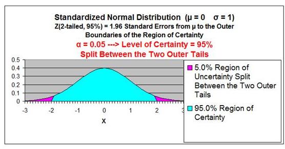
Level of Significance,
α ("alpha"), equals the
maximum allowed percent of error. If the maximum
allowed error is 5%, then α = 0.05.
Level of Confidence is the desired degree of certainty.
A 95% Confidence Level is the most common. A
95% Confidence Level would correspond to a 95
Confidence Interval of the Mean. This would state
that the actual population mean has a 95% probability
of lying within the calculated interval. A 95% Confidence
Level corresponds to a 5% Level of Significance, or
α = 0.05. The Confidence Level therefore equals 1 -
α.
Population Mean = µ ("mu") (This is what we are trying to estimate)
Sample Mean =
xavg
Standard Deviation is a measure of statistical
dispersion. Standard Deviation equals the square root
of the Variance. It's formula is the following:
SQRT ( [ SUM (x -
xavg)2
] / N )
Population Standard Deviation =
σ ("sigma")
Sample Standard Deviation =
s
Standard Error is an estimate of population Standard
Deviation from data taken from a sample. If the population
Standard Deviation, σ, is known, then the Sample Standard
Error, sxavg, can be calculated. If only the Sample Standard
Deviation, s, is known, then Sample Standard Error,
sxavg,
can be estimated by substituting Sample Standard Deviation,
s, for Population Standard Deviation,
σ, as follows:
Sample Standard Error =
sxavg =
σ / SQRT(n)
≈ s / SQRT(n)
σ = Population standard deviation
s = Sample standard deviation
n = sample size
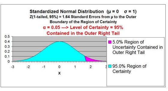
Region of Certainty is the area under the Normal
curve that corresponds to the required Level of Confidence. If a 95% percent Level of Confidence is required, then the
Region of Certainty will contain 95% of the area under the
Normal curve. The outer boundaries of the Region of
Certainty will be the outer boundaries of the Confidence
Interval.
The Region of Certainty, and therefore the Confidence
Interval, will be centered about the mean. Half of the
Confidence Interval is on one side of the mean and
half on the other side.
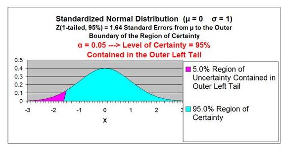
Region of Uncertainty
is the area under the Normal
curve that is outside of the Region of Certainty. Half of the
Region of Uncertainty will exist in the right outer tail of the
Normal curve and the other half in the left outer tail. This is
similar to the concept of the "two-tailed test" that is used in
Hypothesis testing in further sections of this course. The
concepts of one- and two-tailed testing are not used when
calculating Confidence Intervals. Just remember that the
Region of Certainty, and therefore the Confidence Interval,
are always centered about the mean on the Normal curve.
Relationship Between Region of Certainty, Uncertainty, and Alpha
- The Region of Uncertainty corresponds to a ("alpha").
If a = 0.05, then that Region of Uncertainty contains 5%
of the area under the Normal curve. Half of that area
(2.5%) is in each outer tail. The 95% area centered
about the mean will be the Region of Certainty. The
outer boundaries of this Region of Certainty will be
the outer boundaries of the 95% Confidence Interval.
The Level of Confidence is 95% and the Level of
Significance, or maximum error allowed, is 5%.
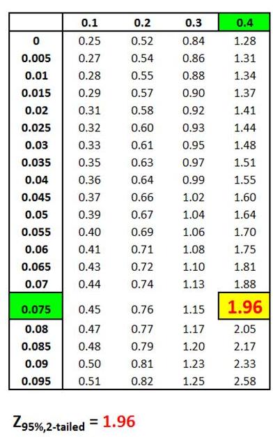
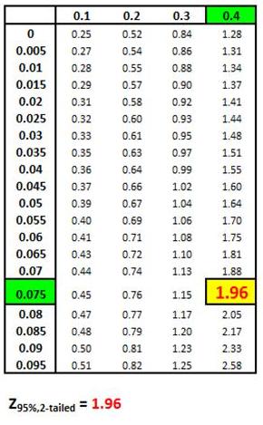
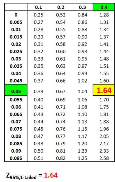
Z Score Chart
Z Score at x (Inner Numbers - Yellow)
vs.
Area Under Normal Curve
Between Mean (µ) and
x (Outer Numbers - Green)
Z Score Chart
Z Score at x (Inner Numbers - Yellow)
vs.
Area Under Normal Curve
Between Mean (µ) and
x (Outer Numbers - Green)
Z Score Chart
Z Score at x (Inner Numbers - Yellow)
vs.
Area Under Normal Curve
Between Mean (µ) and
x (Outer Numbers - Green)
Z Score is the number of Standard Errors from the mean
to outer right boundary of the Region of Certainty (and
therefore to the outer right boundary of the Confidence Interval).
Standard Errors are used and not Standard Deviations
because sample data is being used to calculate the
Confidence Interval.
It is very important to note that on a Standardized Normal Curve, the Distance
from the mean to boundary of the Region of Certainty equals the number of
standard errors from the mean to boundary, which is the Z Score.
The above is only true for a Standardized Normal Curve. It is NOT true for a
Non Standardized Normal curve.
Z Score(1 - α)
= Number of Standard errors from mean to boundary
of Confidence Interval. Note that (1 - α/2) = the entire
area in the Normal curve to the left of outer right boundary
of the Region of Certainty, or Confidence Interval. This
includes the entire Region of Certainty and the half of
the Region of Uncertainty that exists in the left tail.
For example:
Level of Confidence = 95% for a 95% Confidence Interval
Level of Significance (α)= 5%
Two-Tailed Curve
1 - α = 0.95 = 95%
Z Score(95% 2-Tailed) = 1.96
The outer right boundary of the 95% Confidence Interval,
and the Region of Certainty, is 1.96 Standard Errors
from the mean. The left boundary is the same distance
from the mean because the Confidence Interval is
centered about the mean.
Z Score Chart
Z Score at x (Inner Numbers - Yellow)
vs.
Area Under Normal Curve
Between Mean (µ) and
x (Outer Numbers - Green)
The above table indicates that 95% of the area under the
Normal curve lies within 1.96 Standard Errors of the
mean if a two-tailed test is used. This indicates that
2.5% of the total area lies outside 1.96 Standard Errors
of the mean on either side of the mean if a two-tailed
test is used.

The Confidence Interval is the width of the Region of Certainty. The Region
of Certainty extends the same distance from the mean to the left and to the
right because the Normal curve is symmetrical about the mean.
The Confidence Interval extends to the left and to the right of the mean by
the following distance:
Z Score(1-α) * Sample Standard
Error
which equals
Z Score(1-α) *
sxavg
Therefore:
Confidence Interval Boundaries =
= Sample mean +/- Z Score(1-α) * Sample Standard
Error
Confidence Interval Boundaries =
xavg +/- Z Score(1-α) *
sxavg
Confidence Interval Boundaries =
xavg +/- Z Score(1-α)
* σ / SQRT(n)
Confidence Interval Boundaries
≈ xavg +/- Z Score(1-α))
* s / SQRT(n)
As a result of:
Sample Mean = xavg
Sample Standard Deviation =
s
Sample Standard Error =
sxavg
= σ / SQRT(n)
≈ s / SQRT(n)
Sample Size = n
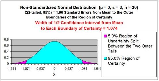
For example, determine the 95% Confidence Interval if the Sample Size is 30,
the Sample Standard Deviation = 3, the sample average = 0, and the
population from which the sample is drawn is Normally Distributed.
α - 1 - 95% = 1 - 0.95 = 0.05
Sample Standard Deviation = s = 3
Sample Size = n = 30
Sample Mean = xavg
= 0
Sample Standard Error =
sxavg
= σ / SQRT(n)
≈ s / SQRT(n) = 3 / SQRT(30)
Sample Standard Error ≈
3 / SQRT(30) =
0.5477
Z Score(1-α)
= Z Score(95%,
2-tailed) = 1.96
Confidence Interval Boundaries =
xavg +/- Z Score(1-α) *
sxavg
Confidence Interval Boundaries
≈
xavg +/- Z Score(1-α)
* s / SQRT(n)
Confidence Interval Boundaries
≈ 0 +/- (1.96) *
(0.5477) = 0 +/- 1.074
Problem: Given the following set of 32 random test scores
taken from a much larger population, calculate with 95%
certainty an interval in which the population mean
test score must fall. In other words, calculate the
95% Confidence Interval for the population test score
mean. The random sample of 32 tests scores is shown
below.
32 Random Test Score Samples from a Much Larger
Population
| 220 |
300 |
| 370 |
410 |
| 500 |
540 |
| 640 |
660 |
| 220 |
300 |
| 370 |
410 |
| 500 |
540 |
| 640 |
660 |
| 220 |
300 |
| 370 |
410 |
| 500 |
540 |
| 640 |
660 |
| 220 |
300 |
| 370 |
410 |
| 500 |
540 |
| 640 |
660 |
Level of Confidence = 95%
= 1 - α
Level of Significance =
α
=
0.05
Sample Size
=
n
=
32
Sample Standard Deviation
=
s
=
149.5
Sample Standard Error =
sxavg
= σ / SQRT(n)
≈ s / SQRT(n) = 149.8 / SQRT(32)
Sample Standard Error ≈
149.8 / SQRT(32) =
26.5
Z Score(1-α)
=
Z Score(95%,
2-tailed) = 1.96
Confidence Interval Boundaries =
xavg +/- Z Score(1-α) *
sxavg
Confidence Interval Boundaries
≈
xavg +/- Z Score(1-α)
* s / SQRT(n)
Confidence Interval Boundaries
≈ 455 +/- (1.96) *
(26.5) = 455 +/- 51.9
Confidence Interval Boundaries
≈ 403.1 to
506.9
Z Score Chart
Z Score at x (Inner Numbers - Yellow)
vs.
Area Under Normal Curve
Between Mean (µ) and
x (Outer Numbers - Green)
This same problem above is solved in the Excel Statistical Master with only 3 Excel formulas (and NO looking anything up on a Z Chart). Everything is explained to you in SIMPLE language in the Excel Statistical Master.
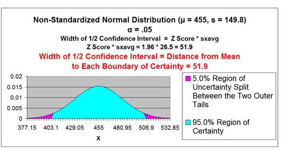
Problem: Average daily demand for books sold in a small
Barnes and Noble store is 455 books with a standard
deviation of 200. This average and standard deviation
are taken from sale data collected every day for a period
of 60 days. What is the range that the true average
daily book sales lies in with 95% certainty?
Level of Confidence = 95% = 1 -
α
Level of Significance =
α = 0.05
Sample Size = n = 60
Sample Mean =
xavg = 455
Sample Standard Deviation =
s = 200
Sample Standard Error =
sxavg
= σ / SQRT(n)
≈ s / SQRT(n)
sxavg =
σ
/ SQRT(n) ≈
s / SQRT(n) = 200 / SQRT(60) = 25.8
Z Score(1 - α)
= Z Score(95% 2-Tailed) = 1.96
Width of Half the Confidence Interval = Z Score(1-α)
* sxavg
Width of Half the Confidence Interval = Z Score(1-α)
* σ / SQRT(n)
Width of Half the Confidence Interval
≈
xavg +/- Z Score(1-α)
* s / SQRT(n)
= 1.96 * 25.8 = 50.6
Confidence Interval Boundaries =
xavg +/- Z Score(1-α) *
sxavg
≈ 455 +/- (1.96)*(25.8) = 455 +/- 50.6 = 404.4 to 505.6
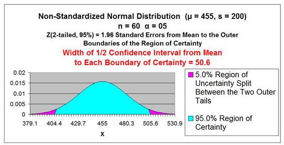
This same problem above is solved in the Excel Statistical Master with only 3 Excel formulas (and not having to look anything up on a Z Chart). The Excel Statistical Master teaches you everything in step-by-step frameworks. You'll never have to memorize any complicated statisical theory.
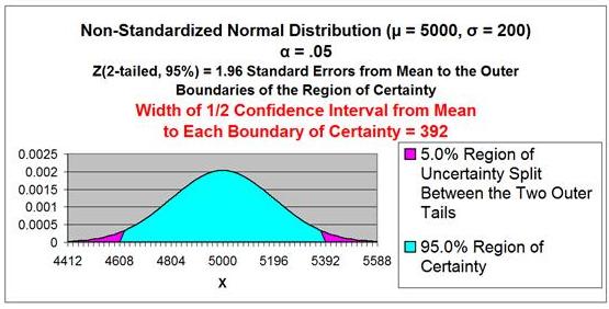
Problem: Average daily demand for books sold in a large
Barnes and Noble store is 5,000 books with a standard
deviation of 200. This average and standard deviation
are taken from sale data collected every day for a
period of 5 years. What is the range that 95% of
the daily unit book sales falls in? The daily sales
data is Normally distributed.
This problem is not a Confidence Interval problem. We do
not need to create an estimate of the population mean
(a Confidence Interval) because we know exactly what
it is. We are given the population mean and population
standard deviation.
We do need to know how the population is distributed
in order to calculate the interval that contains 95% of
all population data. Given that the population is Normally
distributed, we simply need to map the region of this
Normal curve that contains 95% of the total area and
is centered about the mean as follows:
Population mean = µ = 5,000
Population Standard Deviation = σ = 200
Range Containing 95% of Sales Data = µ +/- [
Z Score(95%
2-Tailed) ] *
σ ]
= 5,000 +/- [ 1.96 * 200 ]
= 5,000 +/- 392
= 4,608 to 5,392
Z Score Chart
Z Score at x (Inner Numbers - Yellow)
vs.
Area Under Normal Curve
Between Mean (µ) and
x (Outer Numbers - Green)
This same problem above is solved in the Excel Statistical Master with only 1 Quick Excel formula (and NO looking anything up on a Z Chart). You'll be able to grasp your statistics course a LOT easier with the Excel Statistical Master.
The larger the sample size, the more accurate and tighter
will be the prediction of a population's mean. Stated another
way, the larger the sample size, the smaller will be the
Confidence Interval of the population's mean. Width
of the Confidence Interval is reduced when sample
size is increased.
Quite often a population's mean needs to be estimated with
some level of certainty to within plus or minus a specified
tolerance. This specified tolerance is half the width of the
Confidence Interval. Sample size directly affects the width
of the Confidence Interval. The relationship between sample
size and width of the Confidence Interval is shown as follows:
n = Min Sample Size
Required to Keep Confidence Interval Within a
Required Tolerance
for a Given Confidence Level and
Standard Deviation
Width of Half of the Confidence Interval
= Z Score(1-α) *
σ / SQRT(n)
Width of Half of the Confidence Interval
≈ Z Score(1-α)
* sxavg
As a result of:
Z Score(1-α) *
σ / SQRT(n)
≈ Z Score(1-α) *
s / SQRT(n)
With algebraic manipulation of the above we have:
SQRT(n) = Z Score(1-α) *
σ / Width of Half of the Confidence Interval
n = [ Z Score(1-α) ]2 * [σ]2 / [ Width of Half of the Confidence Interval ]2
Also, if we only have Sample Standard Deviation, s, and not Population
Standard Deviation, σ :
n ≈ [ Z Score(1-α) ]2 * [s]2 / [ Width of Half of the Confidence Interval ]2
Problem 4: Determine the Minimum Number of Sales Territories to Sample
In Order To Limit the 95% Confidence Interval to a Certain Width
Problem: A national sales manager in charge of 5,000
similar territories ran a nationwide promotion. He then
collected sales data from a random sample of the
territories to evaluate sales increase. From the sample,
the average sales increase per territory was $10,000
with a standard deviation of $500. How many territories
would he have had to have sampled to be 95% sure
that the actual nationwide average territory sales
increase was no more than $50 different than average
territory sales increase from the sample he took?
Level of Confidence = 95% = 1 -
α
Level of Significance =
α = 0.05
Sample Size =
n = ?
n = Min Sample Size Required to Keep Confidence
Interval Within a
Required Tolerance
for a Given Confidence Level and
Standard Deviation
Sample Mean =
xavg ------> Note this does not need to be known to solve this problem
Sample Standard Deviation =
s = 500
Z Score(1 - α) =
Z Score(95%
2-Tailed) =
1.96
Width of Half the Confidence Interval
= 50
n ≈ [ Z Score(1-a) ]2 * [s]2 / [ Width of Half of the Confidence Interval ]2
n ≈ [ 1.96 ]2 * [500]2 / [ 50 ]2 = 384
The sales manager would have to sample at least 384 territories
to be 95% certain that nationwide territory average was within
+/- $50 of the sample territory average. Note that the 95%
confidence interval is $10,000 +/- $50 and this interval has a
width = $100 if sample size is 384.
This same problem above is solved in the Excel Statistical Master with only 2 Excel formulas (and not having to look anything up on a Z Chart). If you found your statistics book confusing, You'll really like the Excel Statistical Master. Everything is explained in simple, step-by-step frameworks.
Creating a Confidence Interval for a population's proportion
is very similar to creating a Confidence Interval for a population's
mean. The only real difference is how the standard error is
calculated. Everything else is the same. The method of calculating
a Confidence Interval for a population mean was covered in
detail earlier in this module. First, the difference between
using sampling to estimate a population mean and using
sampling to estimate a population proportion will be explained
below:
What determines whether a mean is being estimated or a
proportion is being estimated is the number of possible
outcomes of each sample taken.
Proportion samples have only two possible outcomes.
For example, if you are comparing the proportion of
Republicans in two different cities, each sample has
only two possible values; the person sampled either
is a Republican or is not.
Mean samples have multiple possible outcomes.
For example, if you are comparing the mean age of
people in two different cities, each sample can have
numerous values; the person sampled could be
anywhere from 1 to 110 years old.
Below is a description of how to calculate a Confidence
Interval for a population's proportion. Note that everything
is almost the same as the calculation of the Confidence
Interval for a mean, except sample standard error.
Level of Significance,
α ("alpha"), equals the maximum
allowed percent of error. If the maximum allowed error is 5%,
then α = 0.05.
Level of Confidence is selected by the user. A 95%
Level is the most common. A 95% Confidence Level would
correspond to a 95% Confidence Interval of the Proportion.
This would state that the actual population Proportion has a 95%probability of lying within the calculated interval. A 95%
Confidence Level corresponds to a 5% Level of Significance,
or α, = 0.05. The Confidence Level therefore equals 1 -
α.
Population Proportion =
µp =
p (This is what we are trying to estimate)
Sample Proportion =
pavg
Standard Deviation is not calculated during the creation of
Confidence Interval for a population proportion.
Standard Error is an estimate of population Standard
Deviation from data taken from a sample. Sample Standard
Error will be an estimate taken from the sample proportion,
pavg, and sample size,
n. This is the major difference
between calculating a Confidence Interval for a proportion
and for a mean. Binomial distribution rules apply to
proportions because a proportion sample has only two
possible outcomes, just like a binomial variable.
Sample Standard Error of a Proportion =
σpavg
σpavg = SQRT(p *
q / n)
≈ spavg
Estimated Sample Standard Error of a Proportion =
spavg
spavg = SQRT (
pavg *
qavg /
n
)
p = Population proportion - This is the unknown that will be estimated with a Confidence Interval
q = 1 -
p
n = Sample Size
pavg = Sample Proportion
qavg = 1 -
pavg
Region of Certainty is the area under the Normal
curve that corresponds to the required Level of Confidence.
If a 95% percent Level of Confidence is required, then the
Region of Certainty will contain 95% of the area under the
Normal curve. The outer boundaries of the Region of
Certainty will be the outer boundaries of the Confidence
Interval.
The Region of Certainty, and therefore the Confidence
Interval, will be centered about the mean. Half of the
Confidence Interval is on one side of the mean and
half on the other side.
Region of Uncertainty is the area under the Normal
curve that is outside of the Region of Certainty. Half of the
Region of Uncertainty will exist in the right outer tail of the
Normal curve and the other half in the left outer tail. This is
similar to the concept of the "two-tailed test" that is used in
Hypothesis testing in further sections of this course. The
concepts of one and two-tailed testing are not used when
calculating Confidence Intervals. Just remember that the
Region of Certainty, and therefore the Confidence Interval,
are always centered about the mean on the Normal curve.
Relationship Between Region of Certainty, Uncertainty, and Alpha
- The Region of Uncertainty corresponds to a ("alpha").
If α = 0.05, then that Region of Uncertainty contains 5%
of the area under the Normal curve. Half of that area
(2.5%) is in each outer tail. The 95% area centered
about the mean will be the Region of Certainty. The
outer boundaries of this Region of Certainty will be
the outer boundaries of the 95% Confidence Interval.
The Level of Confidence is 95% and the Level of
Significance, or maximum error allowed, is 5%.
Z Score is the number of Standard Errors from the mean
to outer right boundary of the Region of Certainty (and
therefore to the outer right boundary of the Confidence Interval).
Standard Errors are used and not Standard Deviations
because sample data is being used to calculate the
Confidence Interval.
It is very important to note that on a Standardized Normal Curve, the Distance
from the mean to boundary of the Region of Certainty equals the number of
standard errors from the mean to boundary, which is the Z Score.
The above is only true for a Standardized Normal Curve. It is NOT true for a
Non Standardized Normal curve.
Z Score(1 - α)
= Number of Standard errors from mean to boundary
of Confidence Interval. Note that (1 - α/2) = the entire
area in the Normal curve to the left of outer right boundary
of the Region of Certainty, or Confidence Interval. This
includes the entire Region of Certainty and the half of
the Region of Uncertainty that exists in the left tail.
For example:
Level of Confidence = 95% for a 95% Confidence Interval
Level of Significance (α)= 5%
Two-Tailed Curve
1 - α = 0.95 = 95%
Z Score(95% 2-Tailed) = 1.96
The outer right boundary of the 95% Confidence Interval,
and the Region of Certainty, is 1.96 Standard Errors
from the mean. The left boundary is the same distance
from the mean because the Confidence Interval is
centered about the mean.
Z Score Chart
Z Score at x (Inner Numbers - Yellow)
vs.
Area Under Normal Curve
Between Mean (µ) and
x (Outer Numbers - Green)
The above table indicates that 95% of the area under the
Normal curve lies within 1.96 Standard Errors of the
mean if a two-tailed test is used. This indicates that
5% of the total area lies outside 1.96 Standard Errors
of the mean in either side of the mean if a two-tailed
test is used.
Confidence Interval Boundaries
= Sample proportion +/- Z Score(1-α) * Sample
Standard Error
Confidence Interval Boundaries
= pavg +/- Z Score(1-α) *
spavg
Sample Proportion =
pavg
Sample Standard Error of a Proportion =
σpavg
≈ spavg
Sample Standard Error of a Proportion
= SQRT ( pavg *
qavg /
n )
Sample size =
n
Confidence Interval Boundaries =
pavg +/- Z Score(1-α) *
spavg
Problem 5: Determine Confidence Interval of Shoppers Who
Prefer to Pay By Credit Card Based Upon Sample Data
Problem: A random sample of 1,000 shoppers was taken.
70% preferred to pay with a credit card. 30% preferred
to pay with cash. Determine the 95% Confidence Interval
for the proportion of the general population that prefers
to pay with a credit card.
Level of Confidence = 95% = 1 -
α
Level of Significance =
α = 0.05
Sample Size = n = 1,000
Sample Proportion =
pavg = 0.70
qavg = 1 -
pavg = 0.30
Sample Standard Error of a Proportion =
σpavg
≈ spavg
spavg = SQRT (
pavg *
qavg /
n )
spavg = SQRT ( 0.70 * 0.30 / 1,000 ) = 0.014
Z Score(1 - α)
= Z Score95% = 1.96
Width of Half the Confidence Interval = Z Score(1-α) *
spavg
= 1.96 * 0.014 = 0.0274
Confidence Interval Boundaries =
pavg +/- Z Score(1-a) *
spavg
= 0.70 +/- (1.96) * (0.014)
= 0.70 +/- 0.0274 = 0.6726 to 0.7274 = 67.26% to 72.74%
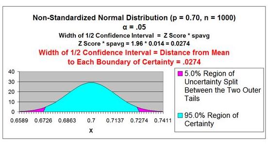
This same problem above is solved in the Excel Statistical Master with only 2 Excel formulas. With the Excel Statistical Master you can do advanced business statistics without having to buy and learn expensive, complicated statistical software packages such as SyStat, MiniTab, SPSS, or SAS.
The larger the sample size, the more accurate and tighter will
be the prediction of a population's mean. Stated another way,
the larger the sample size, the smaller will be the Confidence
Interval of the population's mean. Width of the Confidence
Interval is reduced when sample size is increased.
Quite often a population's mean needs to be estimated with
some level of certainty to within plus or minus a specified
tolerance. This specified tolerance is half the width of the Confidence interval. Sample size directly affects the width
of the Confidence Interval. The relationship between
sample size and width of the Confidence Interval is shown
as follows:
Width of Half the Confidence Interval =Z Score(1-α)*
spavg
spavg = SQRT(
pavg*
qavg/
n)
Width of Half the Confidence Interval = Z Score(1-α)*SQRT(
pavg*
qavg/
n)
[ Width of Half the Confidence Interval ]2 =[Z Score(1-α) ]2*(
pavg*
qavg/
n)
n = [ Z Score(1-α)]2
* ( pavg *
qavg ) / [
Width of Half the Confidence
Interval ]2
Problem 6: Determine the Minimum Sample Size of Voters
to be 95% Certain that the Population Proportion is no more
than 1% Different from Sample Proportion.
Problem: A random survey was conducted in one city to
learn voting preferences. 40% of voters surveyed said
they would vote Republican. 60% of the voters surveyed
said they would vote Democrat. Determine the minimum
number of voters that had to be surveyed to be 95% certain
that the results were accurate within
+/- 1%.
Level of Confidence = 95% = 1 -
α
Level of Significance =
α = 0.05
pavg = 0.40
qavg = 1 -
pavg = 0.60
Width of Half the Confidence Interval = 0.01 ---> (1%)
Z Score(1 - a) = Z Score95%
= 1.96
n = [ Z Score(1-α) ]2 * (
pavg *
qavg ) / [
Width of Half the Confidence
Interval ]2
n = [ 1.96 ]2 * ( 0.40 * 0.60 ) / [ 0.01 ]2 = 9,220
At least 9,220 random voters had to be surveyed to be 95%
certain that the population proportion is no more than 1% different from the
sample.
This same problem above is solved in the Excel Statistical Master with only 2 Excel formulas. The Excel Statistical Master is for you if you want to know how to apply statistics to solve real world business problems.
Copyright 2013