Excel Solver is one of the best and easiest curve-fitting devices in the world, if you know how to use it. Its curve-fitting capabilities make it an excellent tool to perform nonlinear regression. The Excel Solver will find the equation of the linear or nonlinear curve which most closely fits a set of data points.
One very important caveat must be added: the user must first determine the general type of the curve and input that information into Solver at the start. This information is in the form of the general equation that defines the curve, such as a0 + a1*x + a2*x2 = c or a*ln(xb) = c. Solver then calculates all needed variables which produce the equation which most closely fits the data points. We will run through an example here.
In this problem we are going to show how to use the Excel Solver to calculate an equation which most closely describes the relationship between sales and number of ads being run. The purpose of this equation is to be able to predict the number of sales based upon the number of ads that will be run.
A marketing manager has collected this following data on the company’s sales vs. the number of ads that were running at different times.
Sales Number of Ads Running
50 6700
55 7500
59 8700
62 8900
75 8800
95 10900
110 11200
125 11400
140 11500
180 12300
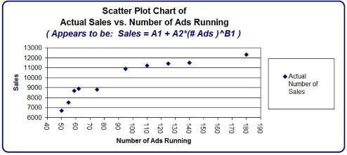
Here is an Excel scatter plot of that data:
We would like to create an equation from this data that allows us to predict the sales based upon the number of ads currently running.
The first step is to eyeball the data and estimate what general type of curve this graph probably is. In this case it appears to a graph the has a diminishing y value for an increasing x value. A formula for such a curve would have the general form:
Y = A1 + A2 * XB1
Sales = A1 + A2 * (Number of Ads Running)B1
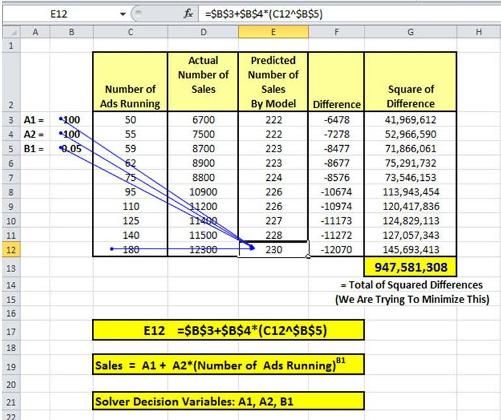
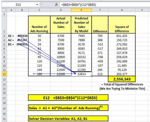
We can use the Excel Solver to solve for A1, A2, and B1. We need to arrange the data in a form that can be input into the Excel Solver as follows:

This table shows the arrangement of data and the calculations. Here we have created an Excel model based upon our model of:
Sales = A1 + A2 * (Number of Ads Running)B1
One example of this formula in action is explained for Cell E16. We are listing the variable that we are solving for (A1, A2, and B1) in cells B3 to B5. In Solver language, these solves that we are changing are called Decision Variables.
We have arbitrarily set our Decision Variables for:
A1 = 100
A2 = 100
B1 = 0.05
We now take the difference between the actual number of sales and the number of sales predicted by our model with our arbitrary settings for the Decision Variables. The square of each difference is taken and then all squares are summed up.
We are trying to find the settings for the Decision Variables that will minimize the sum of the squares of the differences. In other words, we are trying to find A1, A2, and B1 that will minimize the number in cell G13.
Once the Solver has been installed as an add-in (To add-in Solver: File /
Options / Add-Ins / Manage / Excel Add-Ins / Go / Solver Add-In), you can access the Solver in Excel 2010 by: Data / Solver.
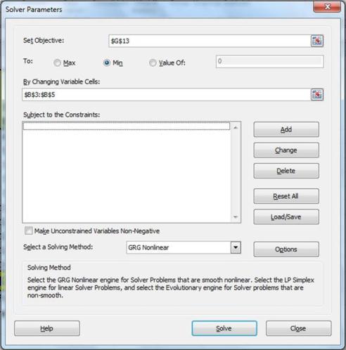
The following blank Solver dialogue box comes up:
![]()
1) The Objective Cell
This is the target cell that we are either trying to maximize, minimize, or achieve a certain value.
2) Minimize or Maximize the Target, or attempt to achieve a certain value in the Objective cell.
3) Decision Variables – A set of variables that will be changed by the Excel Solver in order to optimize the target cell.
4) Constraints – These are the limitations that the problem subjects the Solver to during its calculations
Once again, here is the data table for Solver inputs:
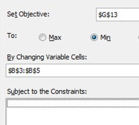
We are trying to minimize Cell G13, the sum of the square of differences between the actual and predicted sales.
We are changing A1, A2, and B1 (cells B3 to B5) to minimize our Objective, Cell G13. The Decision Variables are therefore Cells B3 to B5.
There are none for this curve-fitting operation.
The GRG Nonlinear method is used when the equation producing the objective is not linear but is smooth (continuous). Examples of smooth nonlinear functions in Excel are:
=1/C1, =Log(C1), and =C1^2
These functions have graphs that are curved (nonlinear), but have no breaks (smooth)
Our sales equation appears to be smooth and non-linear:
Sales = A1 + A2 * (Number of Ads Running)B1
Here is the completed Solver dialogue box:
Here is a close-up of the Solver Objective, Decision Variables, and Constraints:
If we now hit the Solve button, we get the following result: Solver has optimized the Decision Variables to minimize the objective function as follows:
A1 = -445,616
A2 = 437,247
B1 = 0.00911
The Objective is minimized to: 2,556,343
We can now create an Excel graph of the Actual Sales vs. the Predicted Sales as follows:
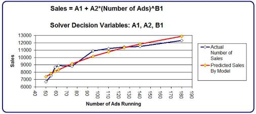
Solver calculates that Sales can be predicted from Number of Ads Running by the following equation:
Sales = -445616 + 437247 * (Number of Ads Running)0.00911
The trickiest part of this problem is the first step; eyeballing the data to determine what kind of graph the data is arranged in. You should take time to evaluate whether you are pursuing calculation of the correct curve type.
You may notice that if you run this problem through the Solver multiple time, you will get slightly different answers. Each time that you run Solver’s GRG algorithm, it will calculate different values for the Decision Variables. You are trying to find the values for the Decision Variables that minimize the objective function (cell G13) the most.
When the Solver runs the GRG algorithm, it picks a starting point for its calculations. Each time you run the Solver GRG method a slightly different starting point will be picked. That is why different answers will appear during each run. Choose the Decision Variable value that occur during the run which produces the lowest value of the Objective. Keep running the Solver until the objective is not minimized anymore. That should give you the optimal values of the Decision Variables. That was done in the example above.
Here are some Solver settings that you want to configure prior to running the Solver for most problems. These settings are found when you click the Options button:
Leave this unchecked. This stops the GRG Solver after each iteration, displaying the result for that iteration. Very rarely is there a reason for doing that.
Leave this box unchecked. You would only use this option if you had reason to believe that inputs of the Solver were measured using different scales.
Only check this if you are sure that none of the variables can ever be negative. In this case, that is clearly not the case.
Leave this box unchecked. There is no advantage to not having Solver reports for each Solver run.
Summary
Excel Solver is an easy-to-use and powerful nonlinear regression tool as a result of its curve-fitting capacity. One use of this is to calculate predictive sales equations for your company. It will work as long as you have properly determined the correct general curve type in the beginning.